Interpretability

ACTL3143 & ACTL5111 Deep Learning for Actuaries

Author

Eric Dong & Patrick Laub

Show the package imports

import random
import matplotlib.pyplot as plt
import numpy as np
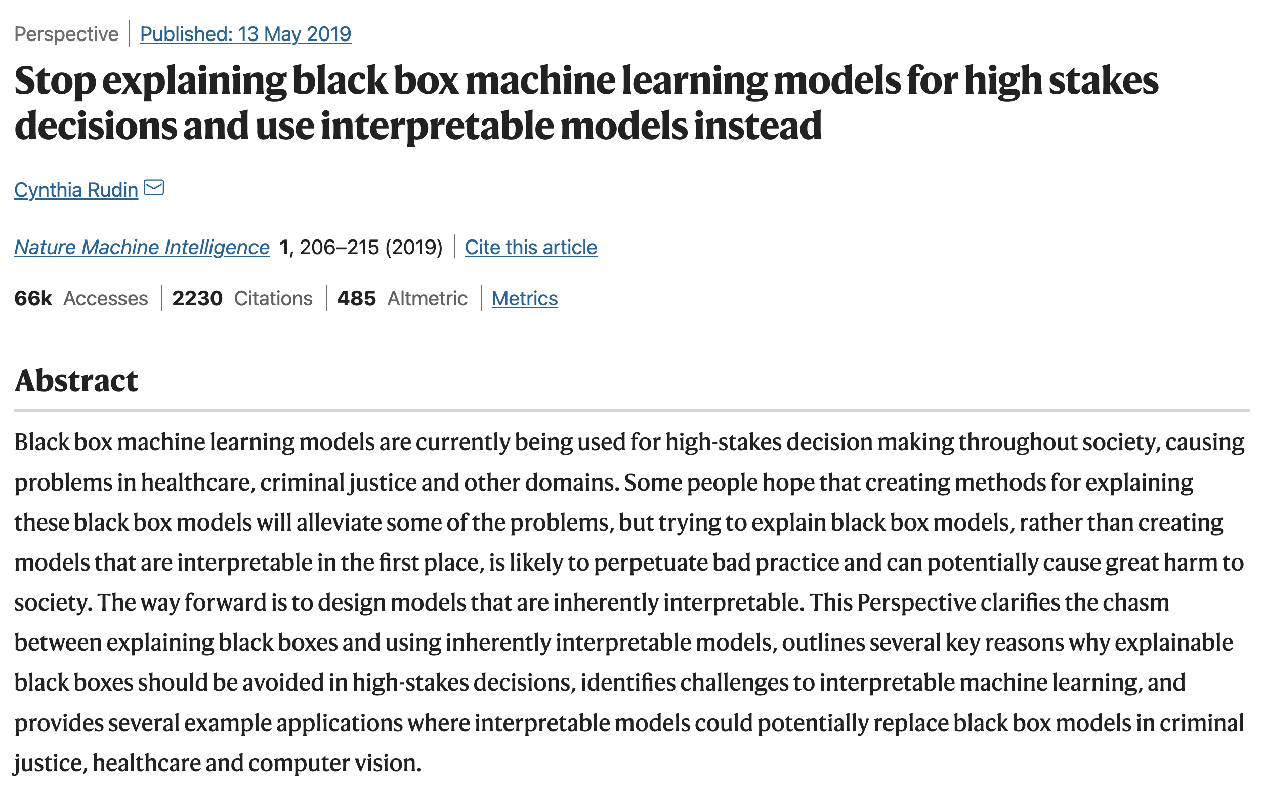
import numpy.random as rnd

Interpretability

Interpretability on a high-level refers to understanding how a model works. Understanding how a model works is very important for decision making. Traditional statistical methods like linear regression and generalized linear regressions are inherently interpretable because we can see and understand how different variables impact the model predictions collectively and individually. In contrast, deep learning algorithms do not readily provide insights into how variables contributed to the predictions. They are composed of multiple layers of interconnected nodes that learn different representations of data. Hence, it is not clear how inputs directly contributed to the outputs. This makes neural networks less interpretable. This is not very desirable, especially in situations which demand making explanations. As such, there is active discussion going on about how we can make less interpretable models more interpretable so that we start trusting these models more.

Interpretability and Trust

Suppose a neural network informs us to increase the premium for Bob.

Why are we getting such a conclusion from the neural network, and should we trust it?
How can we explain our pricing scheme to Bob and the regulators?
Should we be concerned with moral hazards, discrimination, unfairness, and ethical affairs?

We need to trust the model to employ it! With interpretability, we can trust it!

Interpretability

Interpretability Definition: Interpretability refers to the ease with which one can understand and comprehend the model’s algorithm and predictions.

Interpretability of black-box models can be crucial to ascertaining trust.

First Dimension of Interpretability

Inherent Interpretability: The model is interpretable by design.

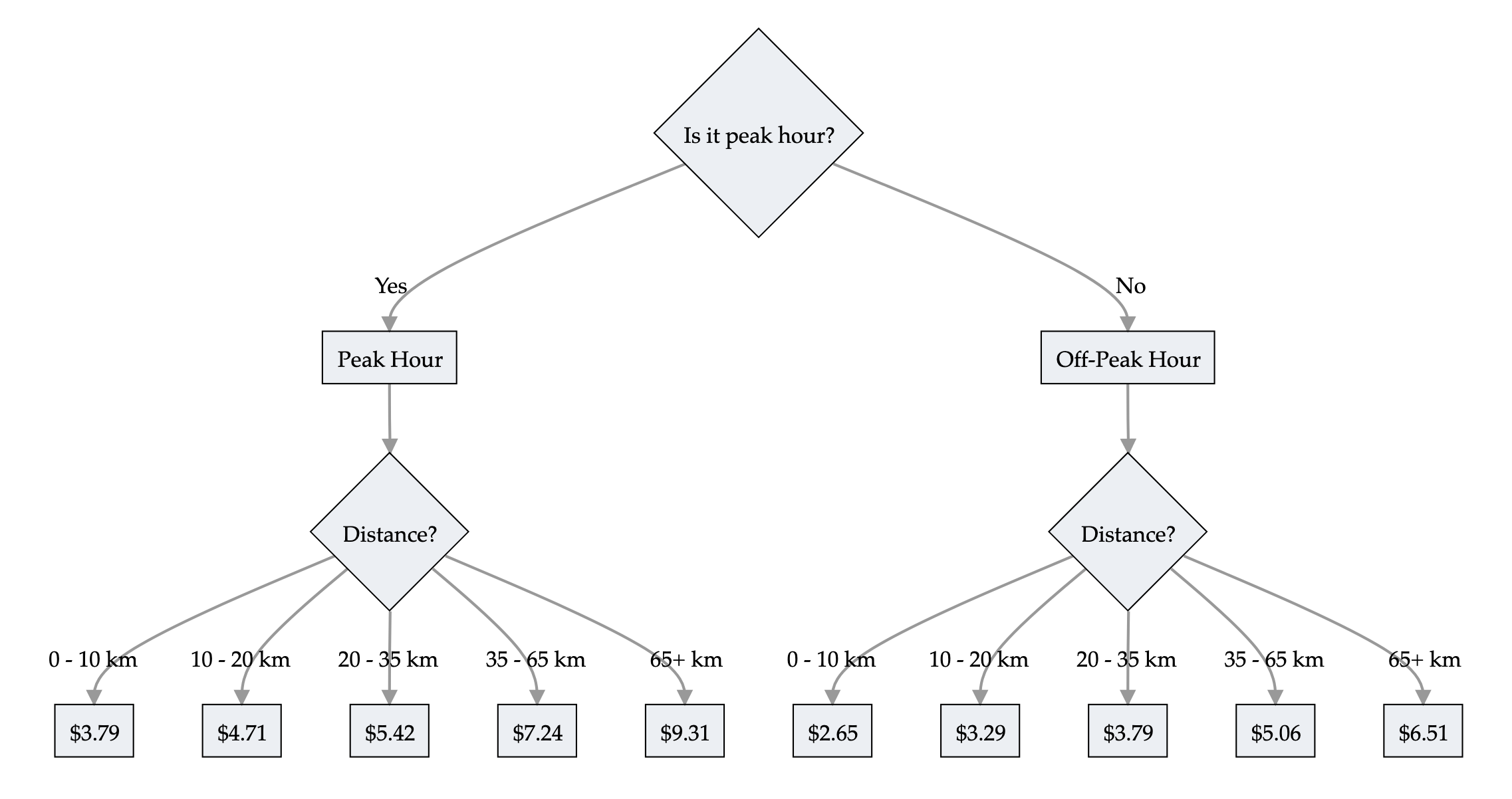
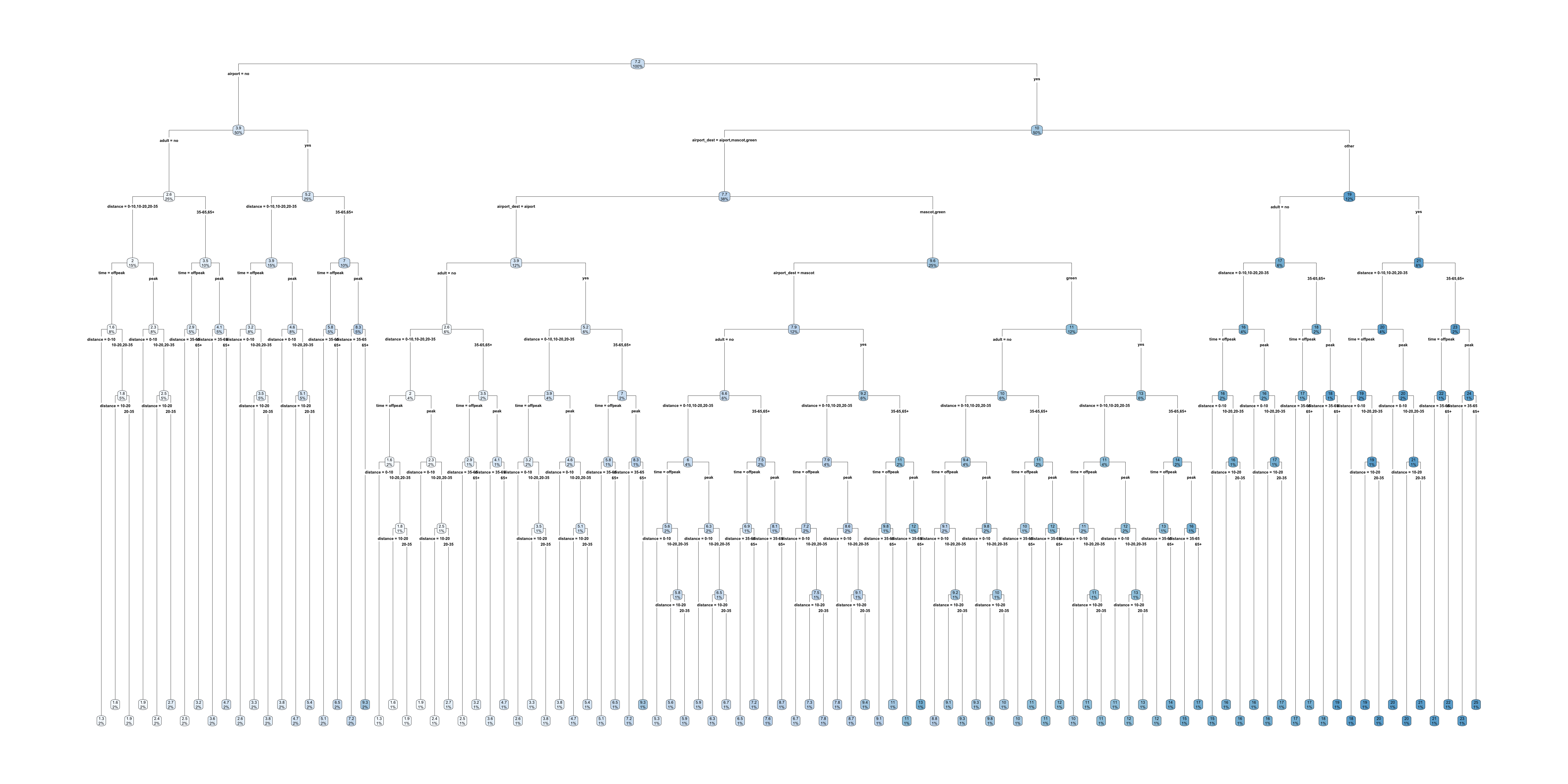
Models with inherent interpretability generally have a simple model architecture where the relationships between inputs and outputs are straightforward. This makes it easy to understand and comprehend model’s inner workings and its predictions. As a result, decision making processes convenient. Examples for models with inherent interpretability include linear regression models, generalized linear regression models and decision trees.

Post-hoc Interpretability: The model is not interpretable by design, but we can use other methods to explain the model.

Post-hoc interpretability refers to applying various techniques to understand how the model makes its predictions after the model is trained. Post-hoc interpretability is useful for understanding predictions coming from complex models (less interpretable models) such as neural networks, random forests and gradient boosting trees.

Second Dimension of Interpretability

Global Interpretability:

The ability to understand how the model works.
Example: how each feature impacts the overall mean prediction.

Global Interpretability focuses on understanding the model’s decision-making process as a whole. Global interpretability takes in to account the entire dataset. These techniques will try to look at general patterns related how input data drives the output in general. Examples for techniques include global feature importance method and permutation importance methods.

Local Interpretability:

The ability to interpret/understand each prediction.
Example: how Bob’s mean prediction has increased the most.

Local Interpretability focuses on understanding the model’s decision-making for a specific input observation. These techniques will try to look at how different input features contributed to the output.

Inherent Interpretability

Trees are interpretable!

Trees are interpretable?

Linear models

A GLM has the form

\hat{y} = g^{-1}\bigl( \beta_0 + \beta_1 x_1 + \dots + \beta_p x_p \bigr)

where \beta_0, \dots, \beta_p are the model parameters.

Global & local interpretations are easy to obtain.

The above GLM representation provides a clear interpretation of how a marginal change in a variable x can contribute to a change in the mean of the output. This makes GLM inherently interpretable.

LocalGLMNet

Imagine: \hat{y_i} = g^{-1}\bigl( \beta_0(\boldsymbol{x}_i) + \beta_1(\boldsymbol{x}_i) x_{i1} + \dots + \beta_p(\boldsymbol{x}_i) x_{ip} \bigr)

A GLM with local parameters \beta_0(\boldsymbol{x}_i), \dots, \beta_p(\boldsymbol{x}_i) for each observation \boldsymbol{x}_i.

The local parameters are the output of a neural network.

Here, \beta_p’s are the neurons from the output layer. First, we define a Feed Foward Neural Network using an input layer, several hidden layers and an output layer. The number of neurons in the output layer must be equal to the number of inputs. Thereafter, we define a skip connection from the input layer directly to the output layer, and merge them using scaler multiplication. Thereafter, the neural network returns the coefficients of the GLM fitted for each individual. We then train the model with the response variable.

Post-hoc Interpretability

Permutation importance

Inputs: fitted model m, tabular dataset D.
Compute the reference score s of the model m on data D (for instance the accuracy for a classifier or the R^2 for a regressor).
For each feature j (column of D):
- For each repetition k in {1, \dots, K}:
  - Randomly shuffle column j of dataset D to generate a corrupted version of the data named \tilde{D}_{k,j}.
  - Compute the score s_{k,j} of model m on corrupted data \tilde{D}_{k,j}.
- Compute importance i_j for feature f_j defined as:
  
  i_j = s - \frac{1}{K} \sum_{k=1}^{K} s_{k,j}

Permutation importance

def permutation_test(model, X, y, num_reps=1, seed=42):
    """
    Run the permutation test for variable importance.
    Returns matrix of shape (X.shape[1], len(model.evaluate(X, y))).
    """
    rnd.seed(seed)
    scores = []    

    for j in range(X.shape[1]):
        original_column = np.copy(X[:, j])
        col_scores = []

        for r in range(num_reps):
            rnd.shuffle(X[:,j])
            col_scores.append(model.evaluate(X, y, verbose=0))

        scores.append(np.mean(col_scores, axis=0))
        X[:,j] = original_column
    
    return np.array(scores)

LIME

Local Interpretable Model-agnostic Explanations employs an interpretable surrogate model to explain locally how the black-box model makes predictions for individual instances.

E.g. a black-box model predicts Bob’s premium as the highest among all policyholders. LIME uses an interpretable model (a linear regression) to explain how Bob’s features influence the black-box model’s prediction.

Globally vs. Locally Faithful

Globally Faithful: The interpretable model’s explanations accurately reflect the behaviour of the black-box model across the entire input space.
Locally Faithful: The interpretable model’s explanations accurately reflect the behaviour of the black-box model for a specific instance.

LIME aims to construct an interpretable model that mimics the black-box model’s behaviour in a locally faithful manner.

LIME Algorithm

Suppose we want to explain the instance \boldsymbol{x}_{\text{Bob}}=(1, 2, 0.5).

Generate perturbed examples of \boldsymbol{x}_{\text{Bob}} and use the trained gamma MDN f to make predictions: \begin{align*} \boldsymbol{x}^{'(1)}_{\text{Bob}} &= (1.1, 1.9, 0.6), \quad f\big(\boldsymbol{x}^{'(1)}_{\text{Bob}}\big)=34000 \\ \boldsymbol{x}^{'(2)}_{\text{Bob}} &= (0.8, 2.1, 0.4), \quad f\big(\boldsymbol{x}^{'(2)}_{\text{Bob}}\big)=31000 \\ &\vdots \quad \quad \quad \quad\quad \quad\quad \quad\quad \quad \quad \vdots \end{align*} We can then construct a dataset of N_{\text{Examples}} perturbed examples: \mathcal{D}_{\text{LIME}} = \big(\big\{\boldsymbol{x}^{'(i)}_{\text{Bob}},f\big(\boldsymbol{x}^{'(i)}_{\text{Bob}}\big)\big\}\big)_{i=0}^{N_{\text{Examples}}}.

LIME Algorithm

Fit an interpretable model g, i.e., a linear regression using \mathcal{D}_{\text{LIME}} and the following loss function: \mathcal{L}_{\text{LIME}}(f,g,\pi_{\boldsymbol{x}_{\text{Bob}}})=\sum_{i=1}^{N_{\text{Examples}}}\pi_{\boldsymbol{x}_{\text{Bob}}}\big(\boldsymbol{x}^{'(i)}_{\text{Bob}}\big)\cdot \bigg(f\big(\boldsymbol{x}^{'(i)}_{\text{Bob}}\big)-g\big(\boldsymbol{x}^{'(i)}_{\text{Bob}}\big)\bigg)^2, where \pi_{\boldsymbol{x}_{\text{Bob}}}\big(\boldsymbol{x}^{'(i)}_{\text{Bob}}\big) represents the distance from the perturbed example \boldsymbol{x}^{'(i)}_{\text{Bob}} to the instance to be explained \boldsymbol{x}_{\text{Bob}}.

“Explaining” to Bob

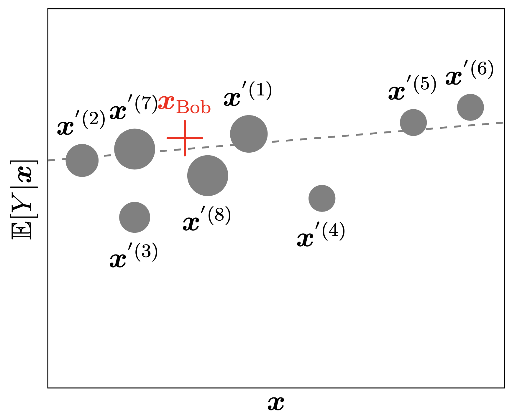
The bold red cross is the instance being explained. LIME samples instances (grey nodes), gets predictions using f (gamma MDN) and weighs them by the proximity to the instance being explained (represented here by size). The dashed line g is the learned local explanation.

SHAP Values

The SHapley Additive exPlanations (SHAP) value helps to quantify the contribution of each feature to the prediction for a specific instance.

The SHAP value for the jth feature is defined as \begin{align*} \text{SHAP}^{(j)}(\boldsymbol{x}) &= \sum_{U\subset \{1, ..., p\} \backslash \{j\}} \frac{1}{p} \binom{p-1}{|U|}^{-1} \big(\mathbb{E}[Y| \boldsymbol{x}^{(U\cup \{j\})}] - \mathbb{E}[Y|\boldsymbol{x}^{(U)}]\big), \end{align*} where p is the number of features. A positive SHAP value indicates that the variable increases the prediction value.

Explaining Specific Models

Grad-CAM

Package Versions

from watermark import watermark
print(watermark(python=True, packages="keras,matplotlib,numpy,pandas,seaborn,scipy,torch,tensorflow,tf_keras"))

Python implementation: CPython
Python version       : 3.11.8
IPython version      : 8.23.0

keras     : 3.2.0
matplotlib: 3.8.4
numpy     : 1.26.4
pandas    : 2.2.1
seaborn   : 0.13.2
scipy     : 1.11.0
torch     : 2.2.2
tensorflow: 2.16.1
tf_keras  : 2.16.0

Glossary

global interpretability
Grad-CAM
inherent interpretability
LIME
local interpretability
permutation importance
post-hoc interpretability
SHAP values