Categorical Variables

ACTL3143 & ACTL5111 Deep Learning for Actuaries

Author

Patrick Laub

Show the package imports
import random
import matplotlib.pyplot as plt
import numpy as np
import pandas as pd

from keras.models import Sequential
from keras.layers import Dense
from keras.callbacks import EarlyStopping

from sklearn.model_selection import train_test_split
from sklearn.preprocessing import OneHotEncoder, StandardScaler
from sklearn.impute import SimpleImputer
from sklearn.linear_model import LinearRegression

Preprocessing

Preprocessing data is essential in creating a successful neural network. Proper preprocessing ensures the data is in a format conducive to learning.

Keras model methods

  • compile: specify the loss function and optimiser
  • fit: learn the parameters of the model
  • predict: apply the model
  • evaluate: apply the model and calculate a metric


random.seed(12)
model = Sequential()
model.add(Dense(1, activation="relu"))
model.compile("adam", "poisson")
model.fit(X_train, y_train, verbose=0)
y_pred = model.predict(X_val, verbose=0)
print(model.evaluate(X_val, y_val, verbose=0))
4.460747718811035

Scikit-learn model methods

  • fit: learn the parameters of the model
  • predict: apply the model
  • score: apply the model and calculate a metric


model = LinearRegression()
model.fit(X_train, y_train)
y_pred = model.predict(X_val)
print(model.score(X_val, y_val))
-0.6668505979514447

Scikit-learn preprocessing methods

  • fit: learn the parameters of the transformation
  • transform: apply the transformation
  • fit_transform: learn the parameters and apply the transformation
scaler = StandardScaler()
scaler.fit(X_train)
X_train_sc = scaler.transform(X_train)
X_val_sc = scaler.transform(X_val)
X_test_sc = scaler.transform(X_test)

print(X_train_sc.mean(axis=0))
print(X_train_sc.std(axis=0))
print(X_val_sc.mean(axis=0))
print(X_val_sc.std(axis=0))
[ 2.97e-17 -1.39e-17  1.98e-17 -5.65e-17]
[1. 1. 1. 1.]
[-0.34  0.07 -0.27 -0.82]
[1.01 0.66 1.26 0.89]
scaler = StandardScaler()
X_train_sc = scaler.fit_transform(X_train)
X_val_sc = scaler.transform(X_val)
X_test_sc = scaler.transform(X_test)

print(X_train_sc.mean(axis=0))
print(X_train_sc.std(axis=0))
print(X_val_sc.mean(axis=0))
print(X_val_sc.std(axis=0))
[ 2.97e-17 -1.39e-17  1.98e-17 -5.65e-17]
[1. 1. 1. 1.]
[-0.34  0.07 -0.27 -0.82]
[1.01 0.66 1.26 0.89]

It is important to make sure that the scaler is fitted using only the data from the train set.

Summary of the splitting

Dataframes & arrays

X_test.head(3)
x1 x2 x3 x4
83 0.075805 -0.677162 0.975120 -0.147057
53 0.954002 0.651391 -0.315269 0.758969
70 0.113517 0.662131 1.586017 -1.237815
X_test_sc
array([[ 0.13, -0.64,  0.89, -0.4 ],
       [ 1.15,  0.67, -0.44,  0.62],
       [ 0.18,  0.68,  1.52, -1.62],
       [ 0.77, -0.82, -1.22,  0.31],
       [ 0.06,  1.46, -0.39,  2.83],
       [ 2.21,  0.49, -1.34,  0.51],
       [-0.57,  0.53, -0.02,  0.86],
       [ 0.16,  0.61, -0.96,  2.12],
       [ 0.9 ,  0.2 , -0.23, -0.57],
       [ 0.62, -0.11,  0.55,  1.48],
       [ 0.  ,  1.57, -2.81,  0.69],
       [ 0.96, -0.87,  1.33, -1.81],
       [-0.64,  0.87,  0.25, -1.01],
       [-1.19,  0.49, -1.06,  1.51],
       [ 0.65,  1.54, -0.23,  0.22],
       [-1.13,  0.34, -1.05, -1.82],
       [ 0.02,  0.14,  1.2 , -0.9 ],
       [ 0.68, -0.17, -0.34,  1.  ],
       [ 0.44, -1.72,  0.22, -0.66],
       [ 0.73,  2.19, -1.13, -0.87],
       [ 2.73, -1.82,  0.59, -2.04],
       [ 1.04, -0.13, -0.13, -1.36],
       [-0.14,  0.43,  1.82, -0.04],
       [-0.24, -0.72, -1.03, -1.15],
       [ 0.28, -0.57, -0.04, -0.66]])

Note

By default, when you pass sklearn a DataFrame it returns a numpy array.

Keep as a DataFrame


From scikit-learn 1.2:

from sklearn import set_config
set_config(transform_output="pandas")

imp = SimpleImputer()
imp.fit(X_train)
X_train_imp = imp.fit_transform(X_train)
X_val_imp = imp.transform(X_val)
X_test_imp = imp.transform(X_test)
  1. Imports set_config function from sklearn.
  2. Sets the configuration to transofrm the output back to pandas.
  3. Defines the SimpleImputer. This function helps in dealing with missing values. Default is set to mean, meaning that, missing values in each column will be replaced with the column mean.
  4. Applies SimpleImputer on the train set before applying the scaler.
  5. Fits and transforms the train set
  6. Transforms the validation set
  7. Transforms the test set
X_test_imp
x1 x2 x3 x4
83 0.075805 -0.677162 0.975120 -0.147057
53 0.954002 0.651391 -0.315269 0.758969
... ... ... ... ...
42 -0.245388 -0.753736 -0.889514 -0.815810
69 0.199060 -0.600217 0.069802 -0.385314

25 rows × 4 columns

French Motor Claims & Poisson Regression

French motor dataset

Download the dataset if we don’t have it already.

from pathlib import Path
from sklearn.datasets import fetch_openml

if not Path("french-motor.csv").exists():
    freq = fetch_openml(data_id=41214, as_frame=True).frame
    freq.to_csv("french-motor.csv", index=False)
else:
    freq = pd.read_csv("french-motor.csv")

freq
IDpol ClaimNb Exposure Area VehPower VehAge DrivAge BonusMalus VehBrand VehGas Density Region
0 1.0 1.0 0.10000 D 5.0 0.0 55.0 50.0 B12 Regular 1217.0 R82
1 3.0 1.0 0.77000 D 5.0 0.0 55.0 50.0 B12 Regular 1217.0 R82
2 5.0 1.0 0.75000 B 6.0 2.0 52.0 50.0 B12 Diesel 54.0 R22
... ... ... ... ... ... ... ... ... ... ... ... ...
678010 6114328.0 0.0 0.00274 D 6.0 2.0 45.0 50.0 B12 Diesel 1323.0 R82
678011 6114329.0 0.0 0.00274 B 4.0 0.0 60.0 50.0 B12 Regular 95.0 R26
678012 6114330.0 0.0 0.00274 B 7.0 6.0 29.0 54.0 B12 Diesel 65.0 R72

678013 rows × 12 columns

  1. Imports Path class from the pathlib.
  2. Imports the fetch_openml function from the sklearn.datasets module. fetch_openml allows the user to bring in the datasets available in the OpenML platform. Every dataset has a unique ID, hence, can be fetched by providing the ID. data_id of the French motor dataset is 41214.
  3. Checks if the dataset does not already exist with in the Jupyter Notebook directory.
  4. Fetches the dataset from OpenML
  5. Convers the dataset into .csv format
  6. If it already exists, then read the dataset as a .csv file

Data dictionary

  • IDpol: policy number (unique identifier)
  • ClaimNb: number of claims on the given policy
  • Exposure: total exposure in yearly units
  • Area: area code (categorical, ordinal)
  • VehPower: power of the car (categorical, ordinal)
  • VehAge: age of the car in years
  • DrivAge: age of the (most common) driver in years
  • BonusMalus: bonus-malus level between 50 and 230 (with reference level 100)
  • VehBrand: car brand (categorical, nominal)
  • VehGas: diesel or regular fuel car (binary)
  • Density: density of inhabitants per km2 in the city of the living place of the driver
  • Region: regions in France (prior to 2016)

The model

Have \{ (\mathbf{x}_i, y_i) \}_{i=1, \dots, n} for \mathbf{x}_i \in \mathbb{R}^{47} and y_i \in \mathbb{N}_0.

Assume the distribution Y_i \sim \mathsf{Poisson}(\lambda(\mathbf{x}_i))

We have \mathbb{E} Y_i = \lambda(\mathbf{x}_i). The NN takes \mathbf{x}_i & predicts \mathbb{E} Y_i.

Note

For insurance, this is a bit weird. The exposures are different for each policy.

\lambda(\mathbf{x}_i) is the expected number of claims for the duration of policy i’s contract.

Normally, \text{Exposure}_i \not\in \mathbf{x}_i, and \lambda(\mathbf{x}_i) is the expected rate per year, then Y_i \sim \mathsf{Poisson}(\text{Exposure}_i \times \lambda(\mathbf{x}_i)).

Where are things defined?

In Keras, string options are used for convenience to reference specific functions or settings.

Meaning that setting activation="relu" (with in strings) is same as setting activation=relu after bringing in the relu function from keras.activations.

model = Sequential([
    Dense(30, activation="relu"),
    Dense(1, activation="exponential")
])

is the same as

from keras.activations import relu, exponential

model = Sequential([
    Dense(30, activation=relu),
    Dense(1, activation=exponential)
])
x = [-1.0, 0.0, 1.0]
print(relu(x))
print(exponential(x))
tensor([0., 0., 1.])
tensor([0.3679, 1.0000, 2.7183])

We can see how relu function gives out x when x is non-negative, and gives out 0 when x is negative. exponential function, takes in x and gives out the exp(x).

String arguments to .compile

When we run

model.compile(optimizer="adam", loss="poisson")

it is equivalent to

from keras.losses import poisson
from keras.optimizers import Adam

model.compile(optimizer=Adam(), loss=poisson)

This is akin to specifying the activation function directly. Setting optimizer="adam" and loss="poisson" as strings is equivalent to using optimizer=Adam() and loss=poisson after importing Adam from keras.optimizers and poisson from keras.losses. Another important thing to note here is that, the loss function is no longer mse. Since we assume a Poisson distribution for the target variable, and the goal is to optimise the algorithm for count data, Poisson loss is more appropriate.

Why do this manually? To adjust the object:

One of the main reasons why we would want to bring in the functions from the libraries (as opposed to using strings) is because it allows us to control the hyper-parameters of the object. For instance, in the example below, we can see how we set the learning_rate to a specific value. learning_rate is an important hyper-parameter in neural network training because it controls the pace at which weights of the neural networks are updated. Too small learning rates can result in slower learning, hence, longer training time. Too large learning rates lead to large steps in weights updates, hence, might miss the optimal solution.

optimizer = Adam(learning_rate=0.01)
model.compile(optimizer=optimizer, loss="poisson")

or to get help.

Keras’ “poisson” loss

help(keras.losses.poisson)
Help on function poisson in module keras.src.losses.losses:

poisson(y_true, y_pred)
    Computes the Poisson loss between y_true and y_pred.
    
    Formula:
    
    ```python
    loss = y_pred - y_true * log(y_pred)
    ```
    
    Args:
        y_true: Ground truth values. shape = `[batch_size, d0, .. dN]`.
        y_pred: The predicted values. shape = `[batch_size, d0, .. dN]`.
    
    Returns:
        Poisson loss values with shape = `[batch_size, d0, .. dN-1]`.
    
    Example:
    
    >>> y_true = np.random.randint(0, 2, size=(2, 3))
    >>> y_pred = np.random.random(size=(2, 3))
    >>> loss = keras.losses.poisson(y_true, y_pred)
    >>> assert loss.shape == (2,)
    >>> y_pred = y_pred + 1e-7
    >>> assert np.allclose(
    ...     loss, np.mean(y_pred - y_true * np.log(y_pred), axis=-1),
    ...     atol=1e-5)

Using the help function in this case provides information about the Poisson loss function in the keras.losses library. It shows that how poisson loss is calculated, by taking two inputs, (i) actual values and (ii) predicted values.

Ordinal Variables

Subsample and split

freq = freq.drop("IDpol", axis=1).head(25_000)

X_train, X_test, y_train, y_test = train_test_split(
  freq.drop("ClaimNb", axis=1), freq["ClaimNb"], random_state=2023)

# Reset each index to start at 0 again.
X_train = X_train.reset_index(drop=True)
X_test = X_test.reset_index(drop=True)
  1. Drops the "IDpol" column and selects only the top 25_000 rows of the dataset
  2. Splits the dataset in to train and test sets. By setting the random_state to a specific number, we ensure the consistency in the train-test split. freq.drop("ClaimNb", axis=1) removes the “ClaimNb” column.
  3. Resets the index of train set, and drops the previous index column. Since the index column will get shuffled during the train-test split, we may want to reset the index to start from 0 again.

What values do we see in the data?

X_train["Area"].value_counts()
X_train["VehBrand"].value_counts()
X_train["VehGas"].value_counts()
X_train["Region"].value_counts()
Area
C    5507
D    4113
A    3527
E    2769
B    2359
F     475
Name: count, dtype: int64
VehBrand
B1     5069
B2     4838
B12    3708
       ... 
B13     336
B11     284
B14     136
Name: count, Length: 11, dtype: int64
VehGas
Regular    10773
Diesel      7977
Name: count, dtype: int64
Region
R24    6498
R82    2119
R11    1909
       ... 
R21      90
R42      55
R43      26
Name: count, Length: 22, dtype: int64

data["column_name"].value_counts() function provides counts of each category for a categorical variable. In this dataset, variables Area and VehGas are assumed to have natural orderings whereas VehBrand and Region are not considered to have such natural orderings. Therefore, the two sets of categorical variables will have to be treated differently.

Ordinal & binary categories are easy

from sklearn.preprocessing import OrdinalEncoder
oe = OrdinalEncoder()
oe.fit(X_train[["Area", "VehGas"]])
oe.categories_
[array(['A', 'B', 'C', 'D', 'E', 'F'], dtype=object),
 array(['Diesel', 'Regular'], dtype=object)]

OrdinalEncoder can assign numerical values to each category of the ordinal variable. The nice thing about OrdinalEncoder is that it can preserve the information about ordinal relationships in the data. Furthermore, this encoding is more efficient in terms of memory usage. 1. Imports the OrdinalEncoder from sklearn.preprocessing library 2. Defines the OrdinalEncoder object as oe 3. Selects the two columns with ordinal variables from X_train and fits the ordinal encoder 4. Gives out the number of unique categories in each ordinal variable

for i, area in enumerate(oe.categories_[0]):
    print(f"The Area value {area} gets turned into {i}.")
The Area value A gets turned into 0.
The Area value B gets turned into 1.
The Area value C gets turned into 2.
The Area value D gets turned into 3.
The Area value E gets turned into 4.
The Area value F gets turned into 5.
for i, gas in enumerate(oe.categories_[1]):
    print(f"The VehGas value {gas} gets turned into {i}.")
The VehGas value Diesel gets turned into 0.
The VehGas value Regular gets turned into 1.

Ordinal encoded values

Note that fitting an ordinal encoder (oe.fit) only establishes the mapping between numerical values and ordinal variable levels. To actually convert the values in the ordinal columns, we must also apply the oe.transform function. Following lines of code shows how we consistently apply the transform function to both train and test sets. To avoid inconsistencies in encoding, we use oe.fit function only to the train set.

X_train_ord = oe.transform(X_train[["Area", "VehGas"]])
X_test_ord = oe.transform(X_test[["Area", "VehGas"]])
X_train[["Area", "VehGas"]].head()
Area VehGas
0 C Diesel
1 C Regular
2 E Regular
3 D Diesel
4 A Regular
X_train_ord.head()
Area VehGas
0 2.0 0.0
1 2.0 1.0
2 4.0 1.0
3 3.0 0.0
4 0.0 1.0

Train on ordinal encoded values

If we would like to see whether we can train a neural network only on the ordinal variables, we can try the following code.

random.seed(12)
model = Sequential([
  Dense(1, activation="exponential")
])

model.compile(optimizer="adam", loss="poisson")

es = EarlyStopping(verbose=True)
hist = model.fit(X_train_ord, y_train, epochs=100, verbose=0,
    validation_split=0.2, callbacks=[es])
hist.history["val_loss"][-1]
Epoch 12: early stopping
0.7823641300201416
  1. Sets the random state for reproducibility
  2. Constructs a neural network with 1 Dense layer, 1 neuron and an exponential activation function
  3. Compiles the model by defining the optimizer and loss function
  4. Defines the early stopping object (Note that the early stopping object only works if we have a validation set. If we do not define a validation set, there will be no validation loss, hence, no metric to compare the training loss with.)
  5. Fits the model only with the encoded columns as input data. The command validation_split=0.2 tells the neural network to treat the last 20% of input data as the validation set. This is an alternative way of defining the validation set.
  6. Returns the validation loss at the final epoch of training


What about adding the continuous variables back in? Use a sklearn column transformer for that.

Preprocess ordinal & continuous

from sklearn.compose import make_column_transformer

ct = make_column_transformer(
  (OrdinalEncoder(), ["Area", "VehGas"]),
  ("drop", ["VehBrand", "Region"]),
  remainder=StandardScaler()
)

X_train_ct = ct.fit_transform(X_train)
  1. Imports the make_column_transformer class that can carry out data preparation selectively
  2. Starts defining the column transformer object
  3. Selects the ordinal columns and apply ordinal encoding
  4. Drops the nominal columns
  5. Applies StandardScaler transformation to the remaining numerical columns
  6. Fits and transforms the train set using the defined column transformer object
X_train.head(3)
Exposure Area VehPower VehAge DrivAge BonusMalus VehBrand VehGas Density Region
0 1.00 C 6.0 2.0 66.0 50.0 B2 Diesel 124.0 R24
1 0.36 C 4.0 10.0 22.0 100.0 B1 Regular 377.0 R93
2 0.02 E 12.0 8.0 44.0 60.0 B3 Regular 5628.0 R11
X_train_ct.head(3)
ordinalencoder__Area ordinalencoder__VehGas remainder__Exposure remainder__VehPower remainder__VehAge remainder__DrivAge remainder__BonusMalus remainder__Density
0 2.0 0.0 1.126979 -0.165005 -0.844589 1.451036 -0.637179 -0.366980
1 2.0 1.0 -0.590896 -1.228181 0.586255 -1.548692 2.303010 -0.302700
2 4.0 1.0 -1.503517 3.024524 0.228544 -0.048828 -0.049141 1.031432

X_train_ct.head(3) returns a dataset with column names replaced according to a strange setting. To avoid that, we can use the verbose_feature_names_out=False command. Following code shows how the command results in a better looking X_train_ct data set.

Preprocess ordinal & continuous II

from sklearn.compose import make_column_transformer

ct = make_column_transformer(
  (OrdinalEncoder(), ["Area", "VehGas"]),
  ("drop", ["VehBrand", "Region"]),
  remainder=StandardScaler(),
  verbose_feature_names_out=False
)
X_train_ct = ct.fit_transform(X_train)
X_train.head(3)
Exposure Area VehPower VehAge DrivAge BonusMalus VehBrand VehGas Density Region
0 1.00 C 6.0 2.0 66.0 50.0 B2 Diesel 124.0 R24
1 0.36 C 4.0 10.0 22.0 100.0 B1 Regular 377.0 R93
2 0.02 E 12.0 8.0 44.0 60.0 B3 Regular 5628.0 R11
X_train_ct.head(3)
Area VehGas Exposure VehPower VehAge DrivAge BonusMalus Density
0 2.0 0.0 1.126979 -0.165005 -0.844589 1.451036 -0.637179 -0.366980
1 2.0 1.0 -0.590896 -1.228181 0.586255 -1.548692 2.303010 -0.302700
2 4.0 1.0 -1.503517 3.024524 0.228544 -0.048828 -0.049141 1.031432

An important thing to notice here is that, the order of columns have changed. They are rearranged according to the order in which we specify the transformations inside the column transformer.

Categorical Variables & Entity Embeddings

Region column

French Administrative Regions

One-hot encoding

oe = OneHotEncoder(sparse_output=False)
X_train_oh = oe.fit_transform(X_train[["Region"]])
X_test_oh = oe.transform(X_test[["Region"]])
print(list(X_train["Region"][:5]))
X_train_oh.head()
['R24', 'R93', 'R11', 'R42', 'R24']
Region_R11 Region_R21 Region_R22 Region_R23 Region_R24 Region_R25 Region_R26 Region_R31 Region_R41 Region_R42 ... Region_R53 Region_R54 Region_R72 Region_R73 Region_R74 Region_R82 Region_R83 Region_R91 Region_R93 Region_R94
0 0.0 0.0 0.0 0.0 1.0 0.0 0.0 0.0 0.0 0.0 ... 0.0 0.0 0.0 0.0 0.0 0.0 0.0 0.0 0.0 0.0
1 0.0 0.0 0.0 0.0 0.0 0.0 0.0 0.0 0.0 0.0 ... 0.0 0.0 0.0 0.0 0.0 0.0 0.0 0.0 1.0 0.0
2 1.0 0.0 0.0 0.0 0.0 0.0 0.0 0.0 0.0 0.0 ... 0.0 0.0 0.0 0.0 0.0 0.0 0.0 0.0 0.0 0.0
3 0.0 0.0 0.0 0.0 0.0 0.0 0.0 0.0 0.0 1.0 ... 0.0 0.0 0.0 0.0 0.0 0.0 0.0 0.0 0.0 0.0
4 0.0 0.0 0.0 0.0 1.0 0.0 0.0 0.0 0.0 0.0 ... 0.0 0.0 0.0 0.0 0.0 0.0 0.0 0.0 0.0 0.0

5 rows × 22 columns

One hot encoding is a way to assign numerical values to nominal variables. One hot encoding is different from ordinal encoding in the way in which it transforms the data. Ordinal encoding assigns a numerical integer to each unique category of the data column and returns one integer column. In contrast, one hot encoding returns a binary vector for each unique category. As a result, what we get from one hot encoding is not a single column vector, but a matrix with number of columns equal to the number of unique categories in that nominal data column.

Train on one-hot inputs

num_regions = len(oe.categories_[0])

random.seed(12)
model = Sequential([
  Dense(2, input_dim=num_regions),
  Dense(1, activation="exponential")
])

model.compile(optimizer="adam", loss="poisson")

es = EarlyStopping(verbose=True)
hist = model.fit(X_train_oh, y_train, epochs=100, verbose=0,
    validation_split=0.2, callbacks=[es])                       
hist.history["val_loss"][-1]
/Users/plaub/miniconda3/envs/ai2024/lib/python3.11/site-packages/keras/src/layers/core/dense.py:86: UserWarning: Do not pass an `input_shape`/`input_dim` argument to a layer. When using Sequential models, prefer using an `Input(shape)` object as the first layer in the model instead.
  super().__init__(activity_regularizer=activity_regularizer, **kwargs)
Epoch 9: early stopping
0.7531585693359375

The above code shows how we can train a neural network using only the one-hot encoded variables. The example is similar to the case of training neural networks for ordinal encoding. 1. Computes the number of unique categories in the encoded column and store it in num_regions 2. Constructs the neural network. This time, it is a neural network with 1 hidden layer and 1 output layer. Dense(2, input_dim=num_regions) takes in an input matrix of with columns = num_regions and transofrmas it down to an output with 2 neurons Steps 3-6 is similar to what we saw during training with ordinal encoded variables.

Consider the first layer

every_category = pd.DataFrame(np.eye(num_regions), columns=oe.categories_[0])
every_category.head(3)
R11 R21 R22 R23 R24 R25 R26 R31 R41 R42 ... R53 R54 R72 R73 R74 R82 R83 R91 R93 R94
0 1.0 0.0 0.0 0.0 0.0 0.0 0.0 0.0 0.0 0.0 ... 0.0 0.0 0.0 0.0 0.0 0.0 0.0 0.0 0.0 0.0
1 0.0 1.0 0.0 0.0 0.0 0.0 0.0 0.0 0.0 0.0 ... 0.0 0.0 0.0 0.0 0.0 0.0 0.0 0.0 0.0 0.0
2 0.0 0.0 1.0 0.0 0.0 0.0 0.0 0.0 0.0 0.0 ... 0.0 0.0 0.0 0.0 0.0 0.0 0.0 0.0 0.0 0.0

3 rows × 22 columns

# Put this through the first layer of the model
X = every_category.to_numpy()
model.layers[0](X)
tensor([[-0.0676, -0.2313],
        [ 0.0578,  0.0541],
        [-0.3354, -0.2603],
        [ 0.0401, -0.3331],
        [ 0.3537, -0.2513],
        [ 0.0741, -0.3928],
        [ 0.2834, -0.3078],
        [ 0.1339,  0.3076],
        [ 0.6641, -0.4717],
        [ 0.2073, -0.0367],
        [-0.0931, -0.4851],
        [ 0.7988, -0.2612],
        [ 0.4994, -0.0385],
        [ 0.7135, -0.3665],
        [-0.2302, -0.1524],
        [-0.2581, -0.0808],
        [ 0.7971,  0.0962],
        [ 0.5428, -0.1990],
        [-0.1908, -0.5027],
        [ 0.1098,  0.1983],
        [ 0.0318,  0.1482],
        [ 0.3183,  0.5048]], grad_fn=<AddBackward0>)

We can extract each layer separately from a trained neural network and observe its output given a specific input. 1. Converts the dataframe to a numpy array 2. Takes out the first layer and feeds in the numpy array X. This returns an array with 2 columns

The first layer

layer = model.layers[0]
W, b = layer.get_weights()
X.shape, W.shape, b.shape
((22, 22), (22, 2), (2,))

We can also extract the layer, get its wieghts and compute manually. 1. Extracts the layer 2. Gets the weights and biases and stores the weights in W and biases in b 3. Returns the shapes of the matrices

X @ W + b
array([[-0.07, -0.23],
       [ 0.06,  0.05],
       [-0.34, -0.26],
       [ 0.04, -0.33],
       [ 0.35, -0.25],
       [ 0.07, -0.39],
       [ 0.28, -0.31],
       [ 0.13,  0.31],
       [ 0.66, -0.47],
       [ 0.21, -0.04],
       [-0.09, -0.49],
       [ 0.8 , -0.26],
       [ 0.5 , -0.04],
       [ 0.71, -0.37],
       [-0.23, -0.15],
       [-0.26, -0.08],
       [ 0.8 ,  0.1 ],
       [ 0.54, -0.2 ],
       [-0.19, -0.5 ],
       [ 0.11,  0.2 ],
       [ 0.03,  0.15],
       [ 0.32,  0.5 ]])
W + b
array([[-0.07, -0.23],
       [ 0.06,  0.05],
       [-0.34, -0.26],
       [ 0.04, -0.33],
       [ 0.35, -0.25],
       [ 0.07, -0.39],
       [ 0.28, -0.31],
       [ 0.13,  0.31],
       [ 0.66, -0.47],
       [ 0.21, -0.04],
       [-0.09, -0.49],
       [ 0.8 , -0.26],
       [ 0.5 , -0.04],
       [ 0.71, -0.37],
       [-0.23, -0.15],
       [-0.26, -0.08],
       [ 0.8 ,  0.1 ],
       [ 0.54, -0.2 ],
       [-0.19, -0.5 ],
       [ 0.11,  0.2 ],
       [ 0.03,  0.15],
       [ 0.32,  0.5 ]], dtype=float32)

The above codes manually compute and returns the same answers as before.

Just a look-up operation

display(list(oe.categories_[0]))
['R11',
 'R21',
 'R22',
 'R23',
 'R24',
 'R25',
 'R26',
 'R31',
 'R41',
 'R42',
 'R43',
 'R52',
 'R53',
 'R54',
 'R72',
 'R73',
 'R74',
 'R82',
 'R83',
 'R91',
 'R93',
 'R94']
W + b
array([[-0.07, -0.23],
       [ 0.06,  0.05],
       [-0.34, -0.26],
       [ 0.04, -0.33],
       [ 0.35, -0.25],
       [ 0.07, -0.39],
       [ 0.28, -0.31],
       [ 0.13,  0.31],
       [ 0.66, -0.47],
       [ 0.21, -0.04],
       [-0.09, -0.49],
       [ 0.8 , -0.26],
       [ 0.5 , -0.04],
       [ 0.71, -0.37],
       [-0.23, -0.15],
       [-0.26, -0.08],
       [ 0.8 ,  0.1 ],
       [ 0.54, -0.2 ],
       [-0.19, -0.5 ],
       [ 0.11,  0.2 ],
       [ 0.03,  0.15],
       [ 0.32,  0.5 ]], dtype=float32)

The above outputs show that the neural network thinks the best way to represent “R11” for this particular problem is using the vector [-0.2, -0.12].

Turn the region into an index

oe = OrdinalEncoder()
X_train_reg = oe.fit_transform(X_train[["Region"]])
X_test_reg = oe.transform(X_test[["Region"]])

for i, reg in enumerate(oe.categories_[0][:3]):
  print(f"The Region value {reg} gets turned into {i}.")
The Region value R11 gets turned into 0.
The Region value R21 gets turned into 1.
The Region value R22 gets turned into 2.

Embedding

from keras.layers import Embedding
num_regions = len(np.unique(X_train[["Region"]]))

random.seed(12)
model = Sequential([
  Embedding(input_dim=num_regions, output_dim=2),
  Dense(1, activation="exponential")
])

model.compile(optimizer="adam", loss="poisson")

Fitting that model

es = EarlyStopping(verbose=True)
hist = model.fit(X_train_reg, y_train, epochs=100, verbose=0,
    validation_split=0.2, callbacks=[es])
hist.history["val_loss"][-1]
Epoch 4: early stopping
0.7527484893798828
model.layers
[<Embedding name=embedding, built=True>, <Dense name=dense_8, built=True>]

Embedding layer can learn the optimal representation for a category of a categorical variable, during training. In the above example, encoding the variable Region using ordinal encoding and passing it through an embedding layer learns the optimal representation for the region during training. Ordinal encoding followed with an embedding layer is a better alternative to one-hot encoding. It is computationally less expensive (compared to generating large matrices in one-hot encoding) particularly when the number of categories is high.

Keras’ Embedding Layer

model.layers[0].get_weights()[0]
array([[ 0.05, -0.08],
       [-0.  ,  0.02],
       [-0.04, -0.02],
       [ 0.11, -0.14],
       [ 0.22, -0.2 ],
       [ 0.15, -0.18],
       [ 0.2 , -0.2 ],
       [-0.04,  0.08],
       [ 0.39, -0.36],
       [ 0.07, -0.06],
       [ 0.08, -0.14],
       [ 0.38, -0.32],
       [ 0.21, -0.15],
       [ 0.37, -0.33],
       [-0.05,  0.01],
       [-0.07,  0.04],
       [ 0.26, -0.16],
       [ 0.27, -0.22],
       [ 0.07, -0.13],
       [-0.  ,  0.04],
       [-0.04,  0.06],
       [-0.04,  0.13]], dtype=float32)
X_train["Region"].head(4)
0    R24
1    R93
2    R11
3    R42
Name: Region, dtype: object
X_sample = X_train_reg[:4].to_numpy()
X_sample
array([[ 4.],
       [20.],
       [ 0.],
       [ 9.]])
enc_tensor = model.layers[0](X_sample)
keras.ops.convert_to_numpy(enc_tensor).squeeze()
array([[ 0.22, -0.2 ],
       [-0.04,  0.06],
       [ 0.05, -0.08],
       [ 0.07, -0.06]], dtype=float32)
  1. Returns the weights of the Embedding layer. The function model.layers[0].get_weights()[0] returns a 22 \times 2 weights matrix with optimal representations for each category. Here 22 corresponds to the number of unique categories, and 2 corresponds to the size of the lower dimensional space using which we represent each category.
  2. Returns the first 4 rows of train set
  3. Converts first 4 rows to a numpy array
  4. Sends the numpy array through the Embedding layer to retrieve corresponding weights We can observe how the last code returns a numpy array with representations corresponding to R24, R93, R11 and R42.

The learned embeddings

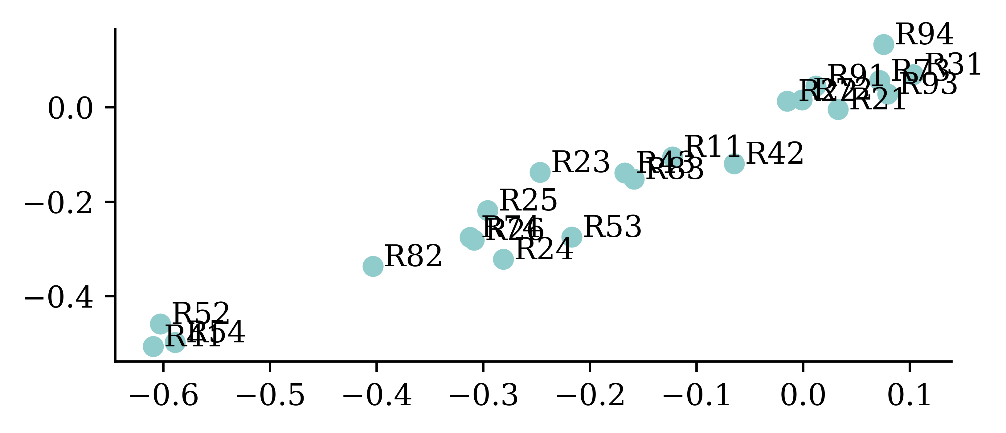
If we only have two-dimensional embeddings we can plot them.

points = model.layers[0].get_weights()[0]
plt.scatter(points[:,0], points[:,1])
for i in range(num_regions):
  plt.text(points[i,0]+0.01, points[i,1] , s=oe.categories_[0][i])

While it not always the case, entity embeddings can at times be meaningful instead of just being useful representations. The above figure shows how plotting the learned embeddings help reveal regions which might be similar (e.g. coastal areas, hilly areas etc.).

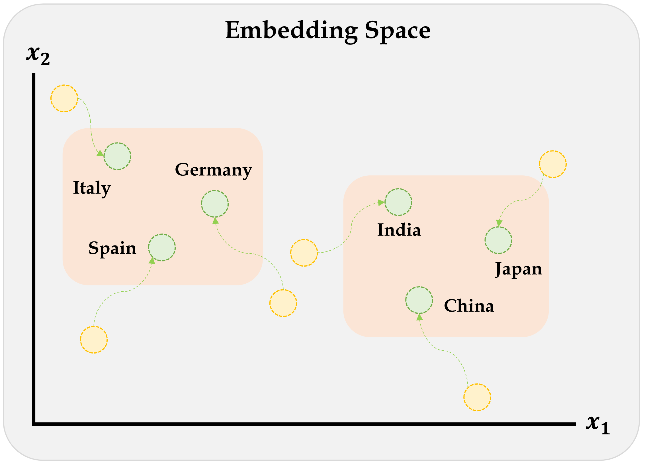
Entity embeddings

Embeddings will gradually improve during training.

Embeddings & other inputs

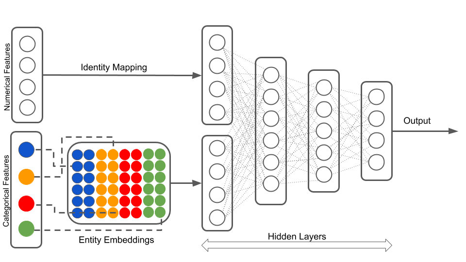
Often times, we deal with both categorical and numerical variables together. The following diagram shows a recommended way of inputting numerical and categorical data in to the neural network. Numerical variables are inherently numeric hence, do not require entity embedding. On the other hand, categorical variables must undergo entity embedding to convert to number format.

Illustration of a neural network with both continuous and categorical inputs.

We can’t do this with Sequential models…

Keras’ Functional API

Sequential models are easy to use and do not require many specifications, however, they cannot model complex neural network architectures. Keras Functional API approach on the other hand allows the users to build complex architectures.

Converting Sequential models

from keras.models import Model
from keras.layers import Input
random.seed(12)

model = Sequential([
  Dense(30, "relu"),
  Dense(1, "exponential")
])

model.compile(
  optimizer="adam",
  loss="poisson")

hist = model.fit(
  X_train_ord, y_train,
  epochs=1, verbose=0,
  validation_split=0.2)
hist.history["val_loss"][-1]
0.805395245552063
random.seed(12)

inputs = Input(shape=(2,))
x = Dense(30, "relu")(inputs)
out = Dense(1, "exponential")(x)
model = Model(inputs, out)

model.compile(
  optimizer="adam",
  loss="poisson")

hist = model.fit(
  X_train_ord, y_train,
  epochs=1, verbose=0,
  validation_split=0.2)
hist.history["val_loss"][-1]
0.805450439453125

Cf. one-length tuples.

The above code shows how to construct the same neural network using sequential models and Keras functional API. There are some differences in the construction. In the functional API approach, we must specify the shape of the input layer, and explicitly define the inputs and outputs of a layer. model = Model(inputs, out) function specifies the input and output of the model. This manner of specifying the inputs and outputs of the model allow the user to combine several inputs (inputs which are preprocessed in different ways) to finally build the model. One example would be combining entity embedded categorical variables, and scaled numerical variables.

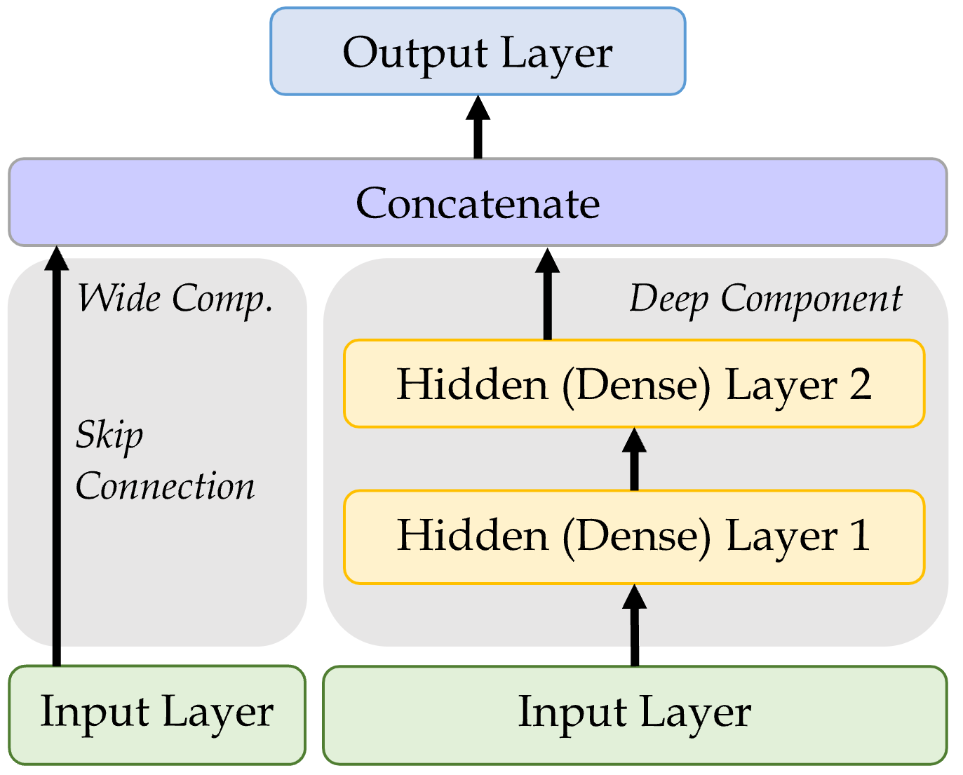
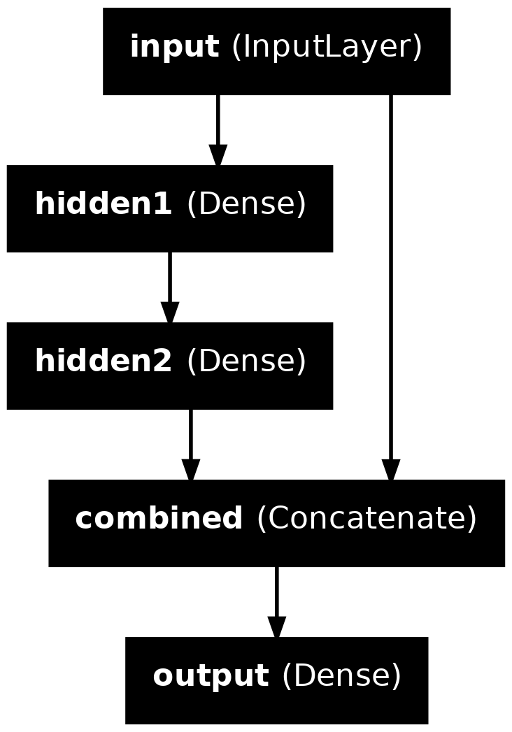
Wide & Deep network

An illustration of the wide & deep network architecture.

Add a skip connection from input to output layers.

from keras.layers \
    import Concatenate

inp = Input(shape=X_train.shape[1:])
hidden1 = Dense(30, "relu")(inp)
hidden2 = Dense(30, "relu")(hidden1)
concat = Concatenate()(
  [inp, hidden2])
output = Dense(1)(concat)
model = Model(
    inputs=[inp],
    outputs=[output])

Naming the layers

For complex networks, it is often useful to give meaningul names to the layers.

input_ = Input(shape=X_train.shape[1:], name="input")
hidden1 = Dense(30, activation="relu", name="hidden1")(input_)
hidden2 = Dense(30, activation="relu", name="hidden2")(hidden1)
concat = Concatenate(name="combined")([input_, hidden2])
output = Dense(1, name="output")(concat)
model = Model(inputs=[input_], outputs=[output])

Inspecting a complex model

from keras.utils import plot_model
plot_model(model, show_layer_names=True)

model.summary(line_length=75)
Model: "functional_10"
┏━━━━━━━━━━━━━━━━━━━━━┳━━━━━━━━━━━━━━━━━━━┳━━━━━━━━━━━┳━━━━━━━━━━━━━━━━━━━┓
┃ Layer (type)         Output Shape         Param #  Connected to      ┃
┡━━━━━━━━━━━━━━━━━━━━━╇━━━━━━━━━━━━━━━━━━━╇━━━━━━━━━━━╇━━━━━━━━━━━━━━━━━━━┩
│ input (InputLayer)  │ (None, 10)        │         0 │ -                 │
├─────────────────────┼───────────────────┼───────────┼───────────────────┤
│ hidden1 (Dense)     │ (None, 30)        │       330 │ input[0][0]       │
├─────────────────────┼───────────────────┼───────────┼───────────────────┤
│ hidden2 (Dense)     │ (None, 30)        │       930 │ hidden1[0][0]     │
├─────────────────────┼───────────────────┼───────────┼───────────────────┤
│ combined            │ (None, 40)        │         0 │ input[0][0],      │
│ (Concatenate)       │                   │           │ hidden2[0][0]     │
├─────────────────────┼───────────────────┼───────────┼───────────────────┤
│ output (Dense)      │ (None, 1)         │        41 │ combined[0][0]    │
└─────────────────────┴───────────────────┴───────────┴───────────────────┘
 Total params: 1,301 (5.08 KB)
 Trainable params: 1,301 (5.08 KB)
 Non-trainable params: 0 (0.00 B)

French Motor Dataset with Embeddings

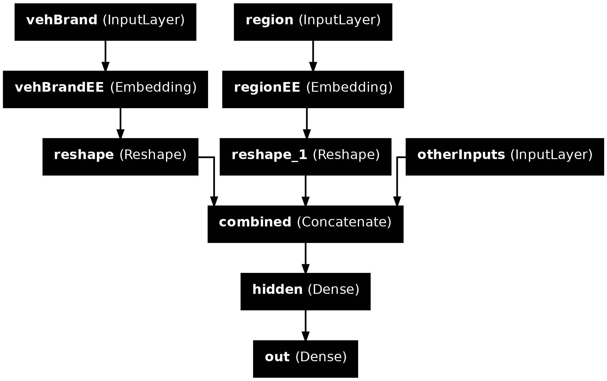
The desired architecture

Illustration of a neural network with both continuous and categorical inputs.

Preprocess all French motor inputs

Transform the categorical variables to integers:

num_brands, num_regions = X_train.nunique()[["VehBrand", "Region"]]

ct = make_column_transformer(
  (OrdinalEncoder(), ["VehBrand", "Region", "Area", "VehGas"]),
  remainder=StandardScaler(),
  verbose_feature_names_out=False
)
X_train_ct = ct.fit_transform(X_train)
X_test_ct = ct.transform(X_test)
  1. Stores separately the number of unique categorical in the nominal variables, as would require these values later for entity embedding
  2. Contructs columns transformer by first ordinally encoding all categorical variables. Ordinal variables are ordinal encoded because it is the sensible thing. Nominal variables are ordinal encoded as an intermediate step before passing through an entity embedding layer
  3. Applies standard scaling to all other numerical variables
  4. verbose_feature_names_out=False stops unnecessarily printing out the outputs of the process
  5. Fits the column transformer to the train set and transforms it
  6. Transforms the test set using the column transformer fitted using the train set

Split the brand and region data apart from the rest:

X_train_brand = X_train_ct["VehBrand"]; X_test_brand = X_test_ct["VehBrand"]
X_train_region = X_train_ct["Region"]; X_test_region = X_test_ct["Region"]
X_train_rest = X_train_ct.drop(["VehBrand", "Region"], axis=1)
X_test_rest = X_test_ct.drop(["VehBrand", "Region"], axis=1)

Organise the inputs

Make a Keras Input for: vehicle brand, region, & others.

veh_brand = Input(shape=(1,), name="vehBrand")
region = Input(shape=(1,), name="region")
other_inputs = Input(shape=X_train_rest.shape[1:], name="otherInputs")

Create embeddings and join them with the other inputs.

from keras.layers import Reshape

random.seed(1337)
veh_brand_ee = Embedding(input_dim=num_brands, output_dim=2,
    name="vehBrandEE")(veh_brand)                                
veh_brand_ee = Reshape(target_shape=(2,))(veh_brand_ee)

region_ee = Embedding(input_dim=num_regions, output_dim=2,
    name="regionEE")(region)
region_ee = Reshape(target_shape=(2,))(region_ee)

x = Concatenate(name="combined")([veh_brand_ee, region_ee, other_inputs])
  1. Imports Reshape class from keras.layers library
  2. Constructs the embedding layer by specifying the input dimension (the number of unique categories) and output dimension (the number of dimensions we want the input to be summarised in to)
  3. Reshapes the output to match the format required at the model building step
  4. Constructs the embedding layer by specifying the input dimension (the number of unique categories) and output dimension
  5. Reshapes the output to match the format required at the model building step
  6. Combines the entity embedded matrices and other inputs together

Complete the model and fit it

Feed the combined embeddings & continuous inputs to some normal dense layers.

x = Dense(30, "relu", name="hidden")(x)
out = Dense(1, "exponential", name="out")(x)

model = Model([veh_brand, region, other_inputs], out)
model.compile(optimizer="adam", loss="poisson")

hist = model.fit((X_train_brand, X_train_region, X_train_rest),
    y_train, epochs=100, verbose=0,
    callbacks=[EarlyStopping(patience=5)], validation_split=0.2)
np.min(hist.history["val_loss"])
0.6694492697715759
  1. Model building stage requires all inputs to be passed in together
  2. Passes in the three sets of data, since the format defined at the model building stage requires 3 data sets

Plotting this model

plot_model(model, show_layer_names=True)

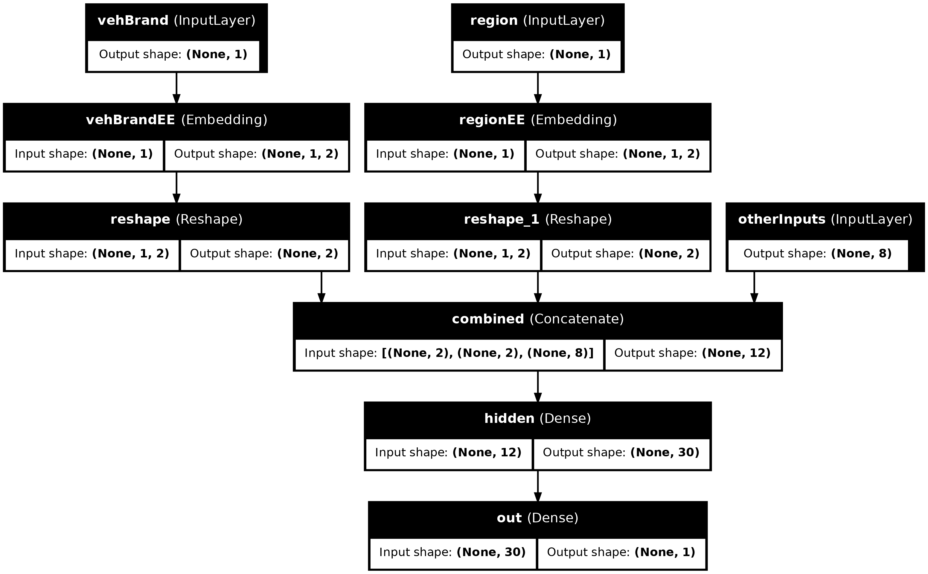
Why we need to reshape

plot_model(model, show_layer_names=True, show_shapes=True)

The plotted model shows how, for example, region starts off as a matrix with (None,1) shape. This indicates that, region was a column matrix with some number of rows. Entity embedding the region variable resulted in a 3D array of shape ((None,1,2)) which is not the required format for concatenating. Therefore, we reshape it using the Reshape function. This results in column array of shape, (None,2) which is what we need for concatenating.

Scale By Exposure

Two different models

Have \{ (\mathbf{x}_i, y_i) \}_{i=1, \dots, n} for \mathbf{x}_i \in \mathbb{R}^{47} and y_i \in \mathbb{N}_0.

Model 1: Say Y_i \sim \mathsf{Poisson}(\lambda(\mathbf{x}_i)).

But, the exposures are different for each policy. \lambda(\mathbf{x}_i) is the expected number of claims for the duration of policy i’s contract.

Model 2: Say Y_i \sim \mathsf{Poisson}(\text{Exposure}_i \times \lambda(\mathbf{x}_i)).

Now, \text{Exposure}_i \not\in \mathbf{x}_i, and \lambda(\mathbf{x}_i) is the rate per year.

Just take continuous variables

For convenience, following code only considers the numerical variables during this implementation.

ct = make_column_transformer(
  ("passthrough", ["Exposure"]),
  ("drop", ["VehBrand", "Region", "Area", "VehGas"]),
  remainder=StandardScaler(),
  verbose_feature_names_out=False
)
X_train_ct = ct.fit_transform(X_train)
X_test_ct = ct.transform(X_test)
  1. Starts defining the column transformer
  2. Lets Exposure passthrough the neural network as it is without peprocessing
  3. Drops the categorical variables (for the ease of implementation)
  4. Scales the remaining variables
  5. Avoids printing unnecessary outputs
  6. Fits and transforms the train set
  7. Only transforms the test set

Split exposure apart from the rest:

X_train_exp = X_train_ct["Exposure"]; X_test_exp = X_test_ct["Exposure"]
X_train_rest = X_train_ct.drop("Exposure", axis=1)
X_test_rest = X_test_ct.drop("Exposure", axis=1)
  1. Takes out Exposure seperately
  2. Drops Exposure from train set
  3. Drops Exposure from test set

Organise the inputs:

exposure = Input(shape=(1,), name="exposure")
other_inputs = Input(shape=X_train_rest.shape[1:], name="otherInputs")

Make & fit the model

Feed the continuous inputs to some normal dense layers.

random.seed(1337)
x = Dense(30, "relu", name="hidden1")(other_inputs)
x = Dense(30, "relu", name="hidden2")(x)
lambda_ = Dense(1, "exponential", name="lambda")(x)
from keras.layers import Multiply

out = Multiply(name="out")([lambda_, exposure])
model = Model([exposure, other_inputs], out)
model.compile(optimizer="adam", loss="poisson")

es = EarlyStopping(patience=10, restore_best_weights=True, verbose=1)
hist = model.fit((X_train_exp, X_train_rest),
    y_train, epochs=100, verbose=0,
    callbacks=[es], validation_split=0.2)
np.min(hist.history["val_loss"])
Epoch 33: early stopping
Restoring model weights from the end of the best epoch: 23.
0.8794452548027039

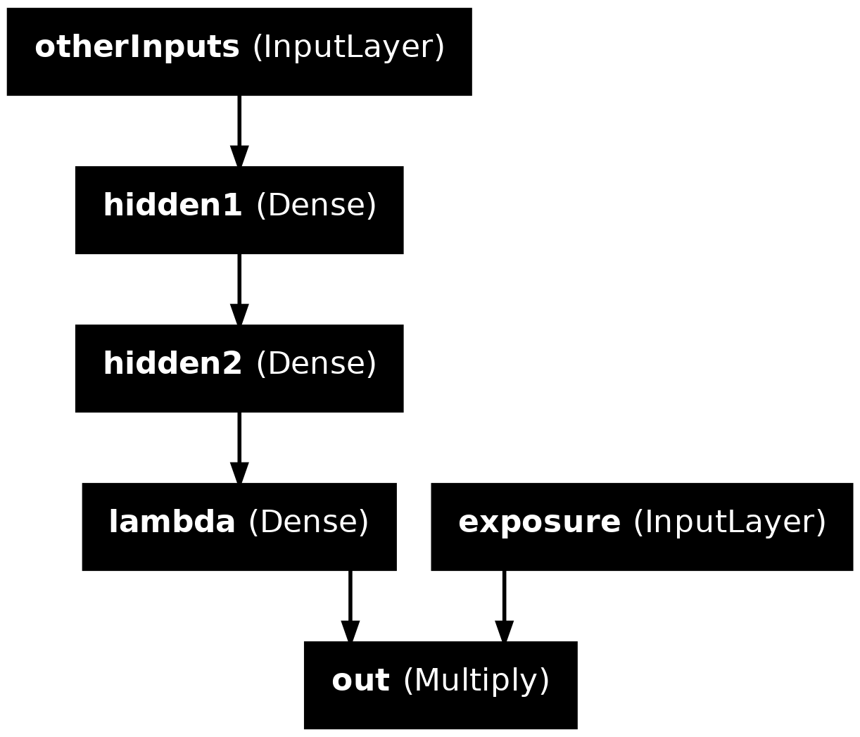
Plot the model

plot_model(model, show_layer_names=True)

Package Versions

from watermark import watermark
print(watermark(python=True, packages="keras,matplotlib,numpy,pandas,seaborn,scipy,torch,tensorflow,tf_keras"))
Python implementation: CPython
Python version       : 3.11.8
IPython version      : 8.23.0

keras     : 3.2.0
matplotlib: 3.8.4
numpy     : 1.26.4
pandas    : 2.2.1
seaborn   : 0.13.2
scipy     : 1.11.0
torch     : 2.2.2
tensorflow: 2.16.1
tf_keras  : 2.16.0

Glossary

  • entity embeddings
  • Input layer
  • Keras functional API
  • Reshape layer
  • skip connection
  • wide & deep network structure