Recurrent Neural Networks

ACTL3143 & ACTL5111 Deep Learning for Actuaries

Author

Patrick Laub

Show the package imports

import random
import matplotlib.pyplot as plt
import numpy as np
import pandas as pd

from keras.models import Sequential
from keras.layers import Dense, Input
from keras.callbacks import EarlyStopping

Tensors & Time Series

Shapes of data

Illustration of tensors of different rank.

The `axis` argument in numpy

Starting with a (3, 4)-shaped matrix:

X = np.arange(12).reshape(3,4)
X

array([[ 0,  1,  2,  3],
       [ 4,  5,  6,  7],
       [ 8,  9, 10, 11]])

The above code creates an array with values from 0 to 11 and converts that array into a matrix with 3 rows and 4 columns.

axis=0: (3, 4) \leadsto (4,).

X.sum(axis=0)

array([12, 15, 18, 21])

The above code returns the column sum. This changes the shape of the matrix from (3,4) to (4,). Similarly, X.sum(axis=1) returns row sums and will change the shape of the matrix from (3,4) to (3,).

axis=1: (3, 4) \leadsto (3,).

X.prod(axis=1)

array([   0,  840, 7920])

The return value’s rank is one less than the input’s rank.

Important

The axis parameter tells us which dimension is removed.

Using `axis` & `keepdims`

With keepdims=True, the rank doesn’t change.

X = np.arange(12).reshape(3,4)
X

array([[ 0,  1,  2,  3],
       [ 4,  5,  6,  7],
       [ 8,  9, 10, 11]])

axis=0: (3, 4) \leadsto (1, 4).

X.sum(axis=0, keepdims=True)

array([[12, 15, 18, 21]])

axis=1: (3, 4) \leadsto (3, 1).

X.prod(axis=1, keepdims=True)

array([[   0],
       [ 840],
       [7920]])

X / X.sum(axis=1)

ValueError: operands could not be broadcast together with shapes (3,4) (3,)

X / X.sum(axis=1, keepdims=True)

array([[0.  , 0.17, 0.33, 0.5 ],
       [0.18, 0.23, 0.27, 0.32],
       [0.21, 0.24, 0.26, 0.29]])

The rank of a time series

Say we had n observations of a time series x_1, x_2, \dots, x_n.

This \mathbf{x} = (x_1, \dots, x_n) would have shape (n,) & rank 1.

If instead we had a batch of b time series’

\mathbf{X} = \begin{pmatrix} x_7 & x_8 & \dots & x_{7+n-1} \\ x_2 & x_3 & \dots & x_{2+n-1} \\ \vdots & \vdots & \ddots & \vdots \\ x_3 & x_4 & \dots & x_{3+n-1} \\ \end{pmatrix} \,,

the batch \mathbf{X} would have shape (b, n) & rank 2.

Multivariate time series

Multivariate time series consists of more than 1 variable observation at a given time point. Following example has two variables x and y.

t	x	y
0	x_0	y_0
1	x_1	y_1
2	x_2	y_2
3	x_3	y_3

Say n observations of the m time series, would be a shape (n, m) matrix of rank 2.

In Keras, a batch of b of these time series has shape (b, n, m) and has rank 3.

Note

Use \mathbf{x}_t \in \mathbb{R}^{1 \times m} to denote the vector of all time series at time t. Here, \mathbf{x}_t = (x_t, y_t).

Some Recurrent Structures

Recurrence relation

A recurrence relation is an equation that expresses each element of a sequence as a function of the preceding ones. More precisely, in the case where only the immediately preceding element is involved, a recurrence relation has the form

u_n = \psi(n, u_{n-1}) \quad \text{ for } \quad n > 0.

Example: Factorial n! = n (n-1)! for n > 0 given 0! = 1.

Diagram of an RNN cell

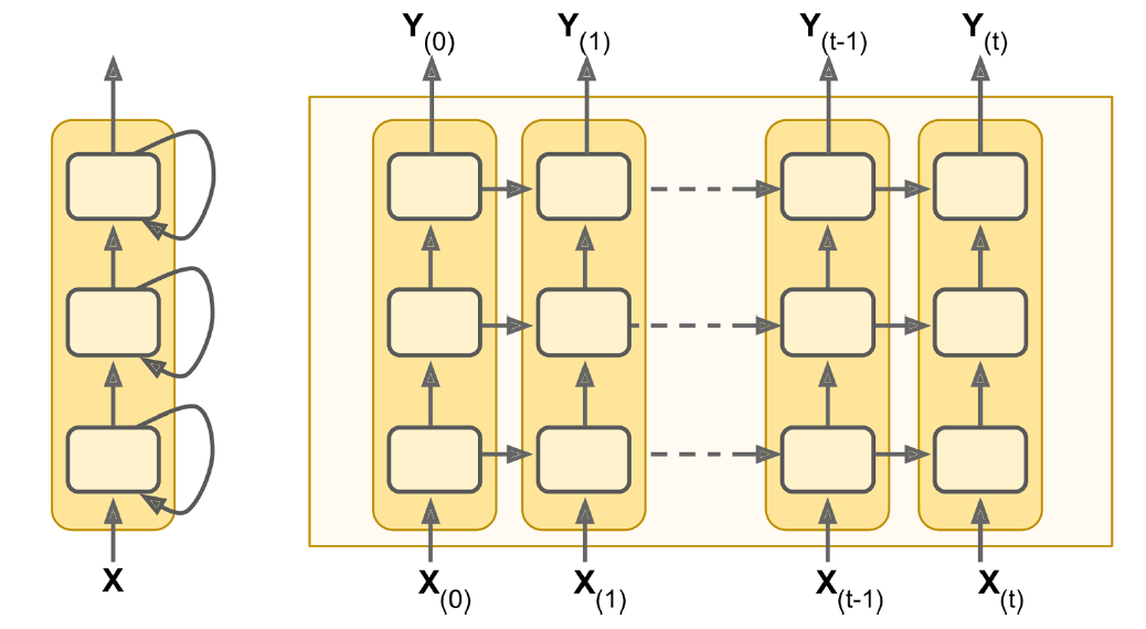
The RNN processes each data in the sequence one by one, while keeping memory of what came before.

The following figure shows how the recurrent neural network combines an input X_l with a preprocessed state of the process A_l to produce the output O_l. RNNs have a cyclic information processing structure that enables them to pass information sequentially from previous inputs. RNNs can capture dependencies and patterns in sequential data, making them useful for analysing time series data.

Schematic of a simple recurrent neural network. E.g. SimpleRNN, LSTM, or GRU.

A SimpleRNN cell.

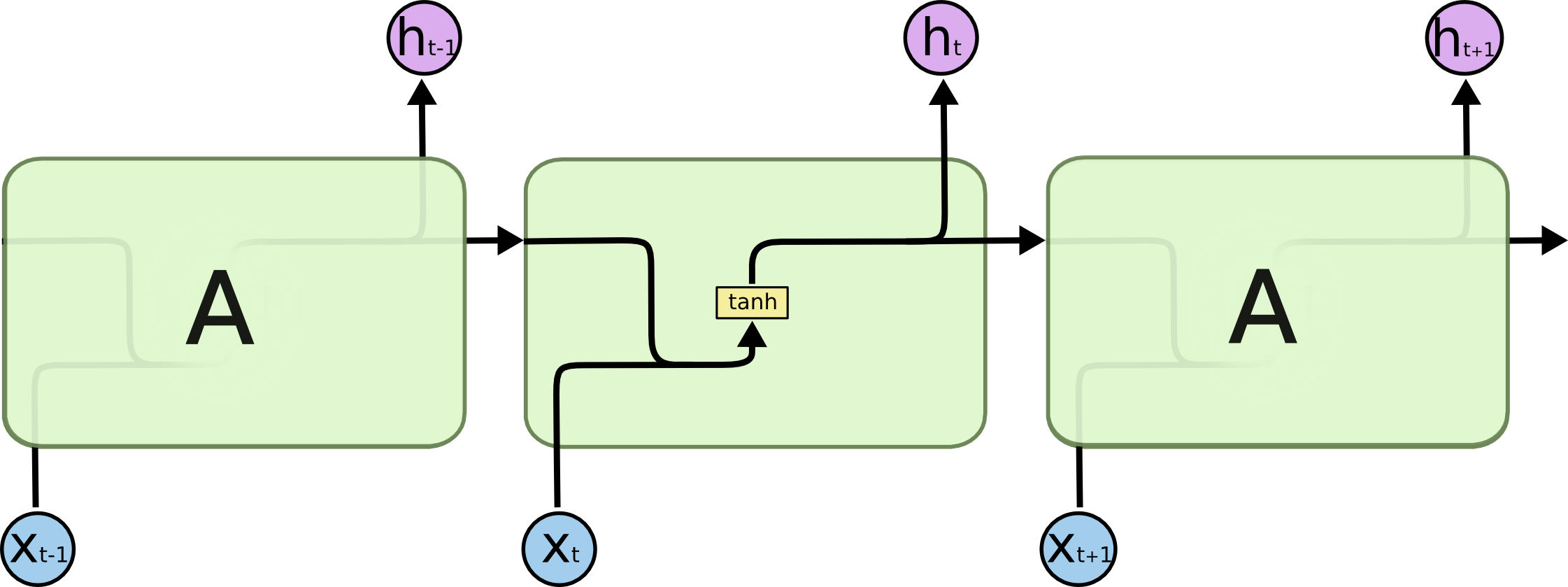
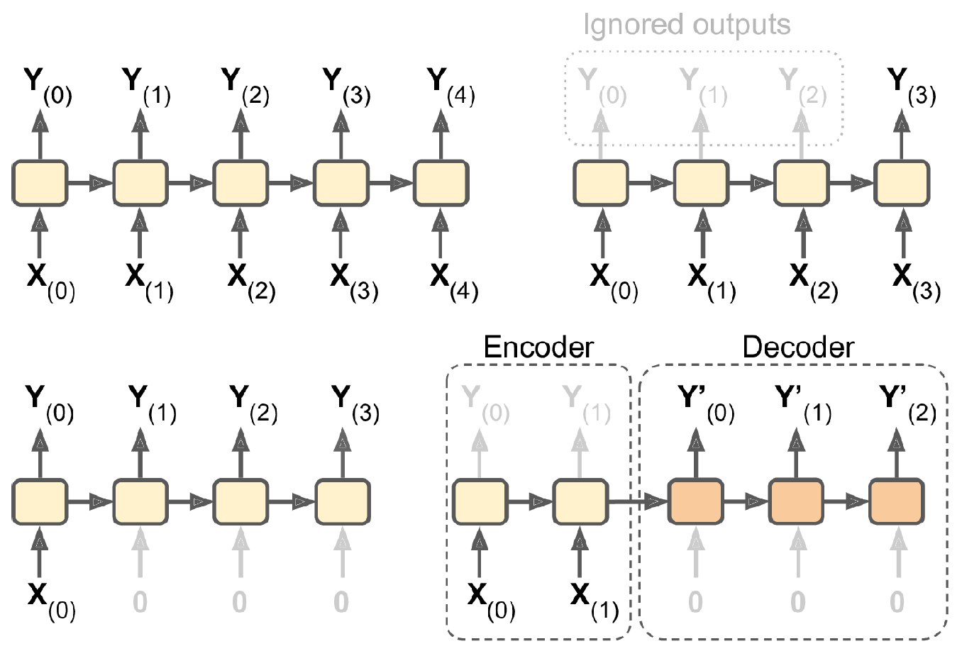
All the outputs before the final one are often discarded.

SimpleRNN

Say each prediction is a vector of size d, so \mathbf{y}_t \in \mathbb{R}^{1 \times d}.

Then the main equation of a SimpleRNN, given \mathbf{y}_0 = \mathbf{0}, is

\mathbf{y}_t = \psi\bigl( \mathbf{x}_t \mathbf{W}_x + \mathbf{y}_{t-1} \mathbf{W}_y + \mathbf{b} \bigr) .

Here, \begin{aligned} &\mathbf{x}_t \in \mathbb{R}^{1 \times m}, \mathbf{W}_x \in \mathbb{R}^{m \times d}, \\ &\mathbf{y}_{t-1} \in \mathbb{R}^{1 \times d}, \mathbf{W}_y \in \mathbb{R}^{d \times d}, \text{ and } \mathbf{b} \in \mathbb{R}^{d}. \end{aligned}

At each time step, a simple Recurrent Neural Network (RNN) takes an input vector x_t, incorporate it with the information from the previous hidden state {y}_{t-1} and produces an output vector at each time step y_t. The hidden state helps the network remember the context of the previous words, enabling it to make informed predictions about what comes next in the sequence. In a simple RNN, the output at time (t-1) is the same as the hidden state at time t.

SimpleRNN (in batches)

The difference between RNN and RNNs with batch processing lies in the way how the neural network handles sequences of input data. With batch processing, the model processes multiple (b) input sequences simultaneously. The training data is grouped into batches, and the weights are updated based on the average error across the entire batch. Batch processing often results in more stable weight updates, as the model learns from a diverse set of examples in each batch, reducing the impact of noise in individual sequences.

Say we operate on batches of size b, then \mathbf{Y}_t \in \mathbb{R}^{b \times d}.

The main equation of a SimpleRNN, given \mathbf{Y}_0 = \mathbf{0}, is \mathbf{Y}_t = \psi\bigl( \mathbf{X}_t \mathbf{W}_x + \mathbf{Y}_{t-1} \mathbf{W}_y + \mathbf{b} \bigr) . Here, \begin{aligned} &\mathbf{X}_t \in \mathbb{R}^{b \times m}, \mathbf{W}_x \in \mathbb{R}^{m \times d}, \\ &\mathbf{Y}_{t-1} \in \mathbb{R}^{b \times d}, \mathbf{W}_y \in \mathbb{R}^{d \times d}, \text{ and } \mathbf{b} \in \mathbb{R}^{d}. \end{aligned}

Simple Keras demo

1num_obs = 4
2num_time_steps = 3
3num_time_series = 2

X = np.arange(num_obs*num_time_steps*num_time_series).astype(np.float32) \
4        .reshape([num_obs, num_time_steps, num_time_series])

output_size = 1                                                                 
y = np.array([0, 0, 1, 1])

1: Defines the number of observations
2: Defines the number of time steps
3: Defines the number of time series
4: Reshapes the array to a range 3 tensor (4,3,2)

1X[:2]

1: Selects the first two slices along the first dimension. Since the tensor of dimensions (4,3,2), X[:2] selects the first two slices (0 and 1) along the first dimension, and returns a sub-tensor of shape (2,3,2).

array([[[ 0.,  1.],
        [ 2.,  3.],
        [ 4.,  5.]],

       [[ 6.,  7.],
        [ 8.,  9.],
        [10., 11.]]], dtype=float32)

1X[2:]

1: Selects the last two slices along the first dimension. The first dimension (axis=0) has size 4. Therefore, X[2:] selects the last two slices (2 and 3) along the first dimension, and returns a sub-tensor of shape (2,3,2).

array([[[12., 13.],
        [14., 15.],
        [16., 17.]],

       [[18., 19.],
        [20., 21.],
        [22., 23.]]], dtype=float32)

Keras’ SimpleRNN

As usual, the SimpleRNN is just a layer in Keras.

1from keras.layers import SimpleRNN

2random.seed(1234)
model = Sequential([
3  SimpleRNN(output_size, activation="sigmoid")
])
4model.compile(loss="binary_crossentropy", metrics=["accuracy"])

5hist = model.fit(X, y, epochs=500, verbose=False)
6model.evaluate(X, y, verbose=False)

1: Imports the SimpleRNN layer from the Keras library
2: Sets the seed for the random number generator to ensure reproducibility
3: Defines a simple RNN with one output node and sigmoid activation function
4: Specifies binary crossentropy as the loss function (usually used in classification problems), and specifies “accuracy” as the metric to be monitored during training
5: Trains the model for 500 epochs and saves output as hist
6: Evaluates the model to obtain a value for the loss and accuracy

[8.05906867980957, 0.5]

The predicted probabilities on the training set are:

model.predict(X, verbose=0)

array([[8.56e-05],
       [2.25e-10],
       [5.98e-16],
       [1.59e-21]], dtype=float32)

SimpleRNN weights

To verify the results of predicted probabilities, we can obtain the weights of the fitted model and calculate the outcome manually as follows.

model.get_weights()

[array([[-1.47],
        [-0.67]], dtype=float32),
 array([[0.99]], dtype=float32),
 array([-0.14], dtype=float32)]

def sigmoid(x):
  return 1 / (1 + np.exp(-x))

W_x, W_y, b = model.get_weights()

Y = np.zeros((num_obs, output_size), dtype=np.float32)
for t in range(num_time_steps):
    X_t = X[:, t, :]
    z = X_t @ W_x + Y @ W_y + b
    Y = sigmoid(z)

Y

array([[8.56e-05],
       [2.25e-10],
       [5.98e-16],
       [1.59e-21]], dtype=float32)

LSTM internals

Simple RNN structures encounter vanishing gradient problems, hence, struggle with learning long term dependencies. LSTM are designed to overcome this problem. LSTMs have a more complex network structure (contains more memory cells and gating mechanisms) and can better regulate the information flow.

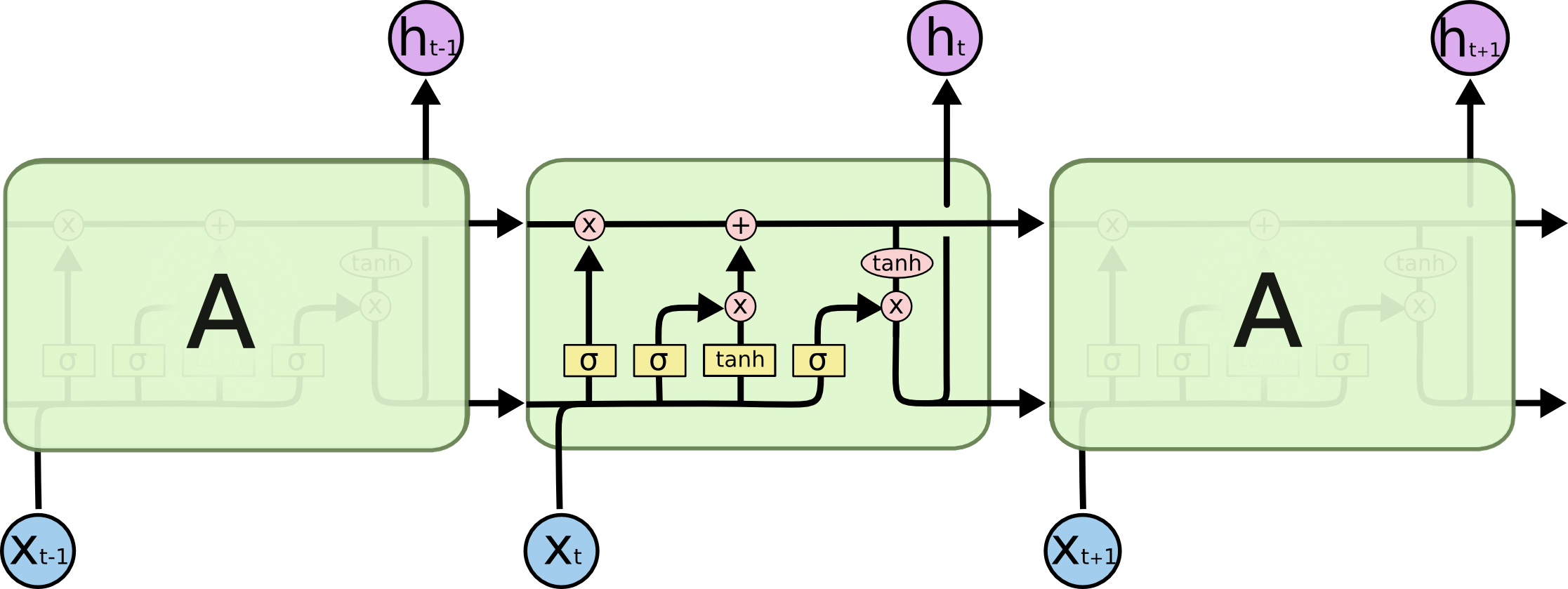
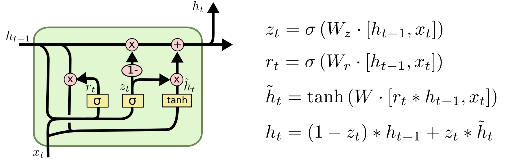
Diagram of an LSTM cell. Notation for the diagram.

GRU internals

GRUs are simpler compared to LSTM, hence, computationally more efficient than LSTMs.

Recurrent Neural Networks

Basic facts of RNNs

A recurrent neural network is a type of neural network that is designed to process sequences of data (e.g. time series, sentences).
A recurrent neural network is any network that contains a recurrent layer.
A recurrent layer is a layer that processes data in a sequence.
An RNN can have one or more recurrent layers.
Weights are shared over time; this allows the model to be used on arbitrary-length sequences.

Applications

Forecasting: revenue forecast, weather forecast, predict disease rate from medical history, etc.
Classification: given a time series of the activities of a visitor on a website, classify whether the visitor is a bot or a human.
Event detection: given a continuous data stream, identify the occurrence of a specific event. Example: Detect utterances like “Hey Alexa” from an audio stream.
Anomaly detection: given a continuous data stream, detect anything unusual happening. Example: Detect unusual activity on the corporate network.

Input and output sequences

Categories of recurrent neural networks: sequence to sequence, sequence to vector, vector to sequence, encoder-decoder network.

Input and output sequences

Sequence to sequence: Useful for predicting time series such as using prices over the last N days to output the prices shifted one day into the future (i.e. from N-1 days ago to tomorrow.)
Sequence to vector: ignore all outputs in the previous time steps except for the last one. Example: give a sentiment score to a sequence of words corresponding to a movie review.

Input and output sequences

Vector to sequence: feed the network the same input vector over and over at each time step and let it output a sequence. Example: given that the input is an image, find a caption for it. The image is treated as an input vector (pixels in an image do not follow a sequence). The caption is a sequence of textual description of the image. A dataset containing images and their descriptions is the input of the RNN.
The Encoder-Decoder: The encoder is a sequence-to-vector network. The decoder is a vector-to-sequence network. Example: Feed the network a sequence in one language. Use the encoder to convert the sentence into a single vector representation. The decoder decodes this vector into the translation of the sentence in another language.

Recurrent layers can be stacked.

CoreLogic Hedonic Home Value Index

Australian House Price Indices

Percentage changes

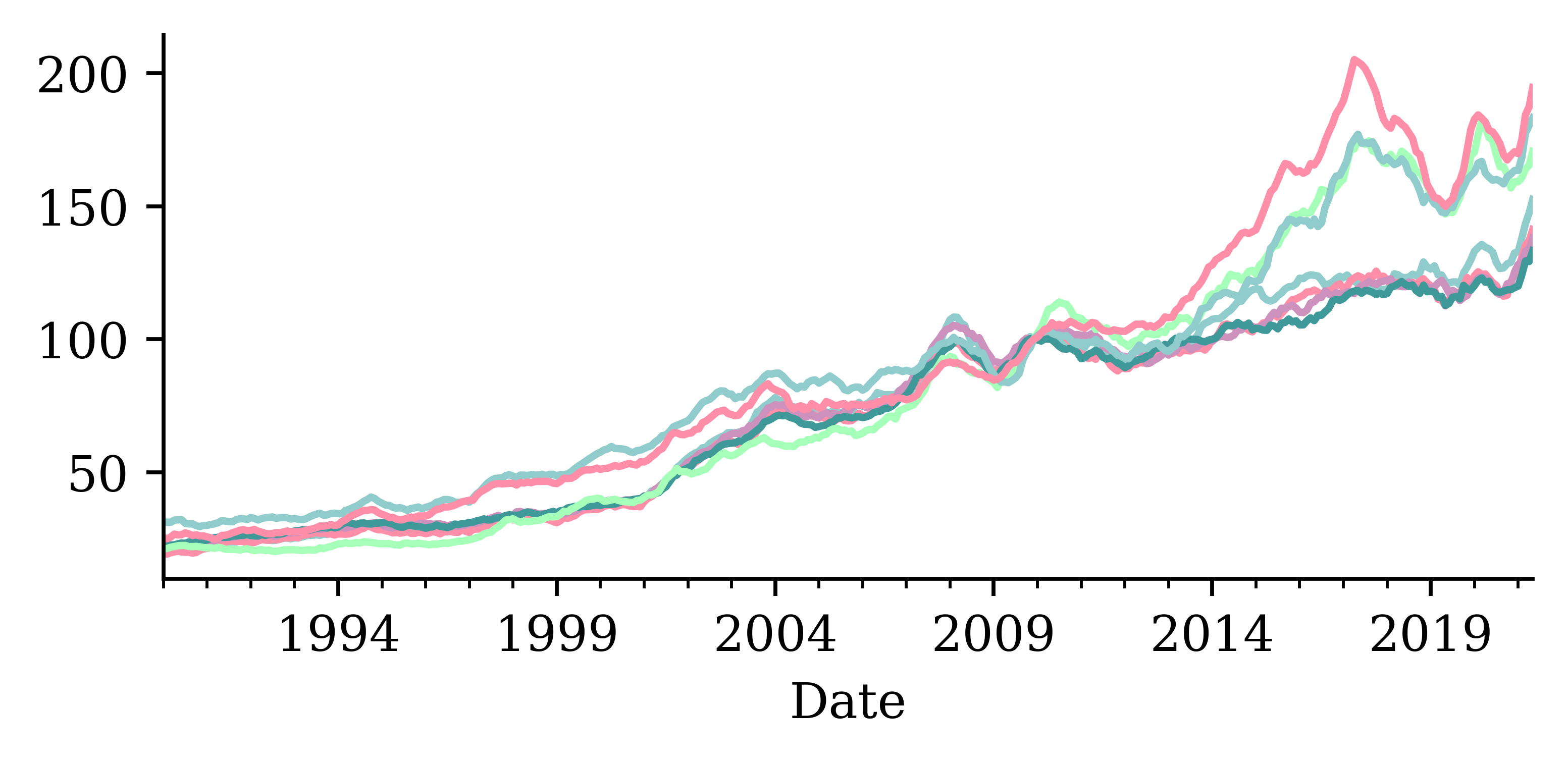
changes = house_prices.pct_change().dropna()
changes.round(2)

	Brisbane	East_Bris	North_Bris	West_Bris	Melbourne	North_Syd	Sydney
Date
1990-02-28	0.03	-0.01	0.01	0.01	0.00	-0.00	-0.02
1990-03-31	0.01	0.03	0.01	0.01	0.02	-0.00	0.03
...	...	...	...	...	...	...	...
2021-04-30	0.03	0.01	0.01	-0.00	0.01	0.02	0.02
2021-05-31	0.03	0.03	0.03	0.03	0.03	0.02	0.04

376 rows × 7 columns

Percentage changes

changes.plot();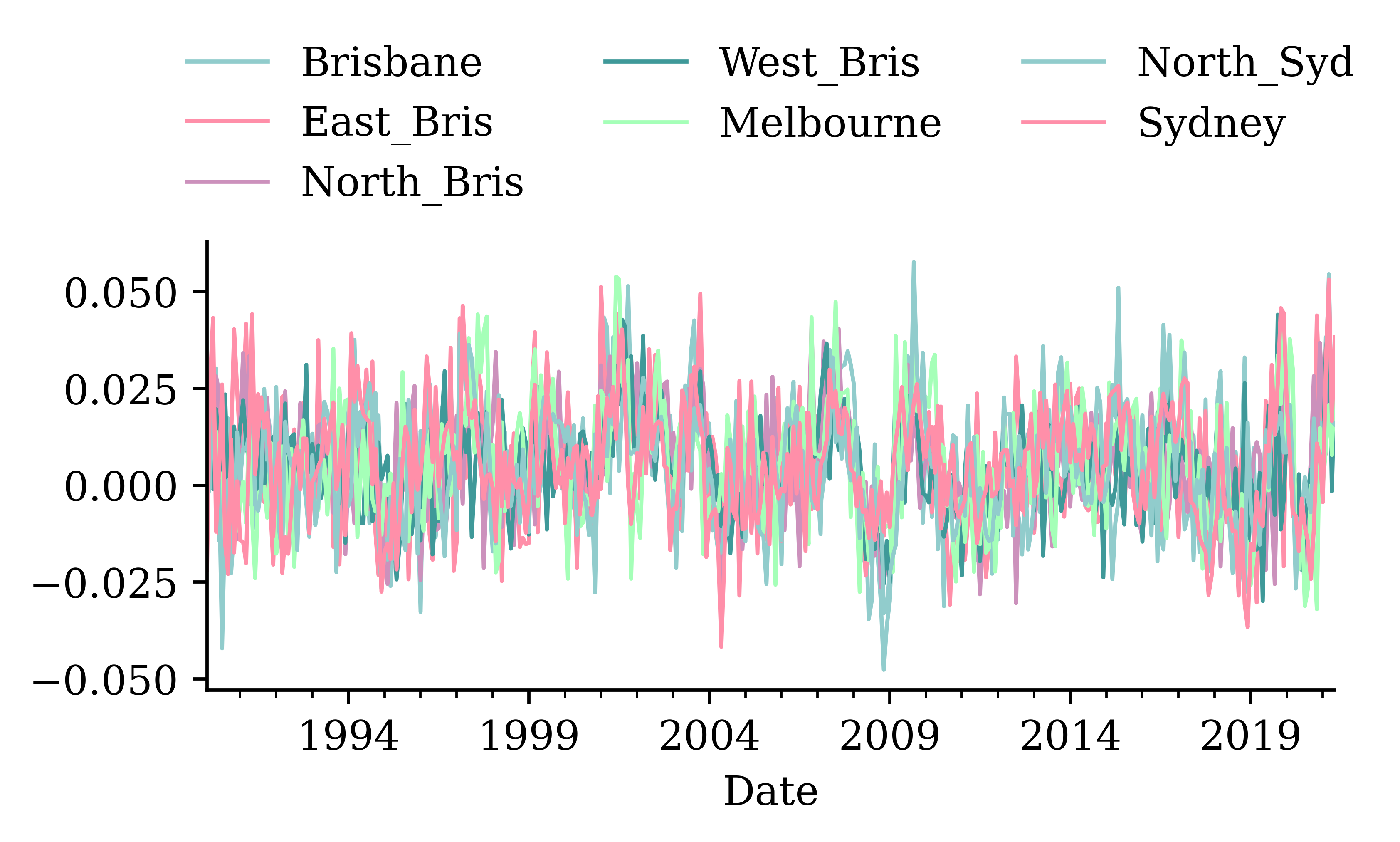

The size of the changes

changes.mean()

Brisbane      0.005496
East_Bris     0.005416
North_Bris    0.005024
West_Bris     0.004842
Melbourne     0.005677
North_Syd     0.004819
Sydney        0.005526
dtype: float64

changes *= 100

changes.mean()

Brisbane      0.549605
East_Bris     0.541562
North_Bris    0.502390
West_Bris     0.484204
Melbourne     0.567700
North_Syd     0.481863
Sydney        0.552641
dtype: float64

changes.plot(legend=False);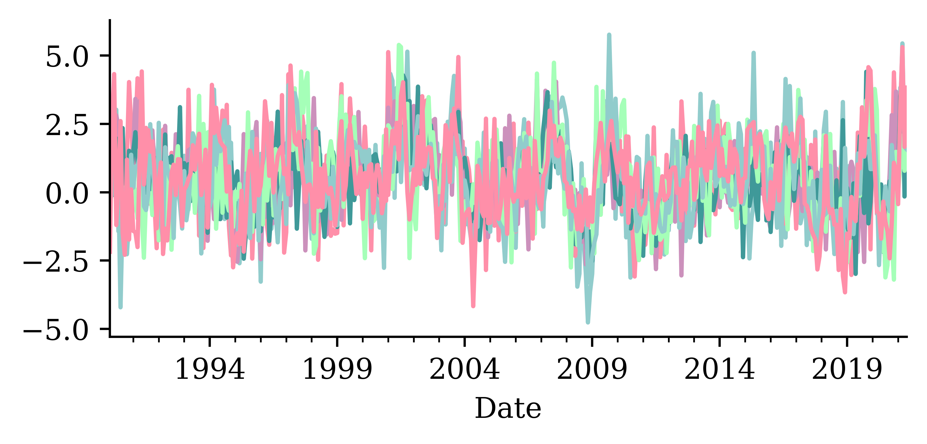

Splitting time series data

Split without shuffling

num_train = int(0.6 * len(changes))
num_val = int(0.2 * len(changes))
num_test = len(changes) - num_train - num_val
print(f"# Train: {num_train}, # Val: {num_val}, # Test: {num_test}")

# Train: 225, # Val: 75, # Test: 76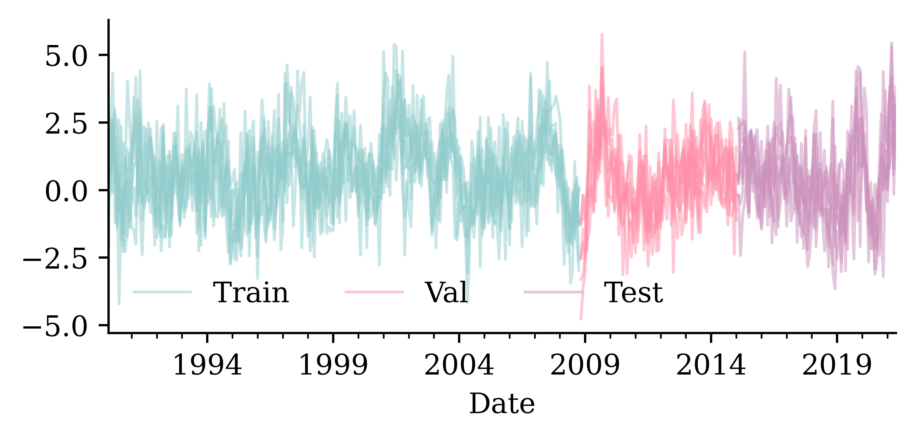

Subsequences of a time series

Keras has a built-in method for converting a time series into subsequences/chunks.

from keras.utils import timeseries_dataset_from_array

integers = range(10)                                
dummy_dataset = timeseries_dataset_from_array(
    data=integers[:-3],                                 
    targets=integers[3:],                               
    sequence_length=3,                                      
    batch_size=2,                                           
)

for inputs, targets in dummy_dataset:
    for i in range(inputs.shape[0]):
        print([int(x) for x in inputs[i]], int(targets[i]))

[0, 1, 2] 3
[1, 2, 3] 4
[2, 3, 4] 5
[3, 4, 5] 6
[4, 5, 6] 7

On time series splits

If you have a lot of time series data, then use:

from keras.utils import timeseries_dataset_from_array
data = range(20); seq = 3; ts = data[:-seq]; target = data[seq:]
nTrain = int(0.5 * len(ts)); nVal = int(0.25 * len(ts))
nTest = len(ts) - nTrain - nVal
print(f"# Train: {nTrain}, # Val: {nVal}, # Test: {nTest}")

# Train: 8, # Val: 4, # Test: 5

trainDS = \
  timeseries_dataset_from_array(
    ts, target, seq,
    end_index=nTrain)

valDS = \
  timeseries_dataset_from_array(
    ts, target, seq,
    start_index=nTrain,
    end_index=nTrain+nVal)

testDS = \
  timeseries_dataset_from_array(
    ts, target, seq,
    start_index=nTrain+nVal)

Training dataset
[0, 1, 2] 3
[1, 2, 3] 4
[2, 3, 4] 5
[3, 4, 5] 6
[4, 5, 6] 7
[5, 6, 7] 8

Validation dataset
[8, 9, 10] 11
[9, 10, 11] 12

Test dataset
[12, 13, 14] 15
[13, 14, 15] 16
[14, 15, 16] 17

On time series splits II

If you don’t have a lot of time series data, consider:

X = []; y = []
for i in range(len(data)-seq):
    X.append(data[i:i+seq])
    y.append(data[i+seq])
X = np.array(X); y = np.array(y);

nTrain = int(0.5 * X.shape[0])
X_train = X[:nTrain]
y_train = y[:nTrain]

nVal = int(np.ceil(0.25 * X.shape[0]))
X_val = X[nTrain:nTrain+nVal]
y_val = y[nTrain:nTrain+nVal]

nTest = X.shape[0] - nTrain - nVal
X_test = X[nTrain+nVal:]
y_test = y[nTrain+nVal:]

Training dataset
[0, 1, 2] 3
[1, 2, 3] 4
[2, 3, 4] 5
[3, 4, 5] 6
[4, 5, 6] 7
[5, 6, 7] 8
[6, 7, 8] 9
[7, 8, 9] 10

Validation dataset
[8, 9, 10] 11
[9, 10, 11] 12
[10, 11, 12] 13
[11, 12, 13] 14
[12, 13, 14] 15

Test dataset
[13, 14, 15] 16
[14, 15, 16] 17
[15, 16, 17] 18
[16, 17, 18] 19

Predicting Sydney House Prices

Creating dataset objects

# Num. of input time series.
num_ts = changes.shape[1]

# How many prev. months to use.
seq_length = 6

# Predict the next month ahead.
ahead = 1

# The index of the first target.
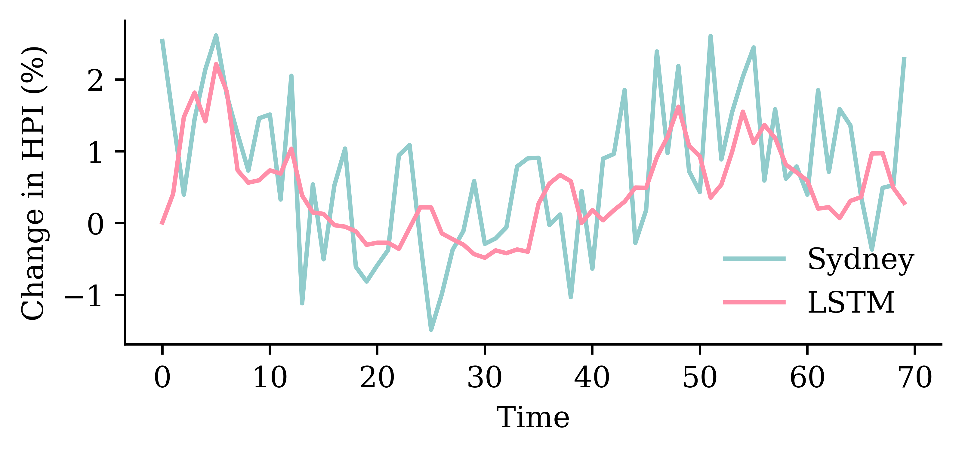
delay = (seq_length+ahead-1)

# Which suburb to predict.
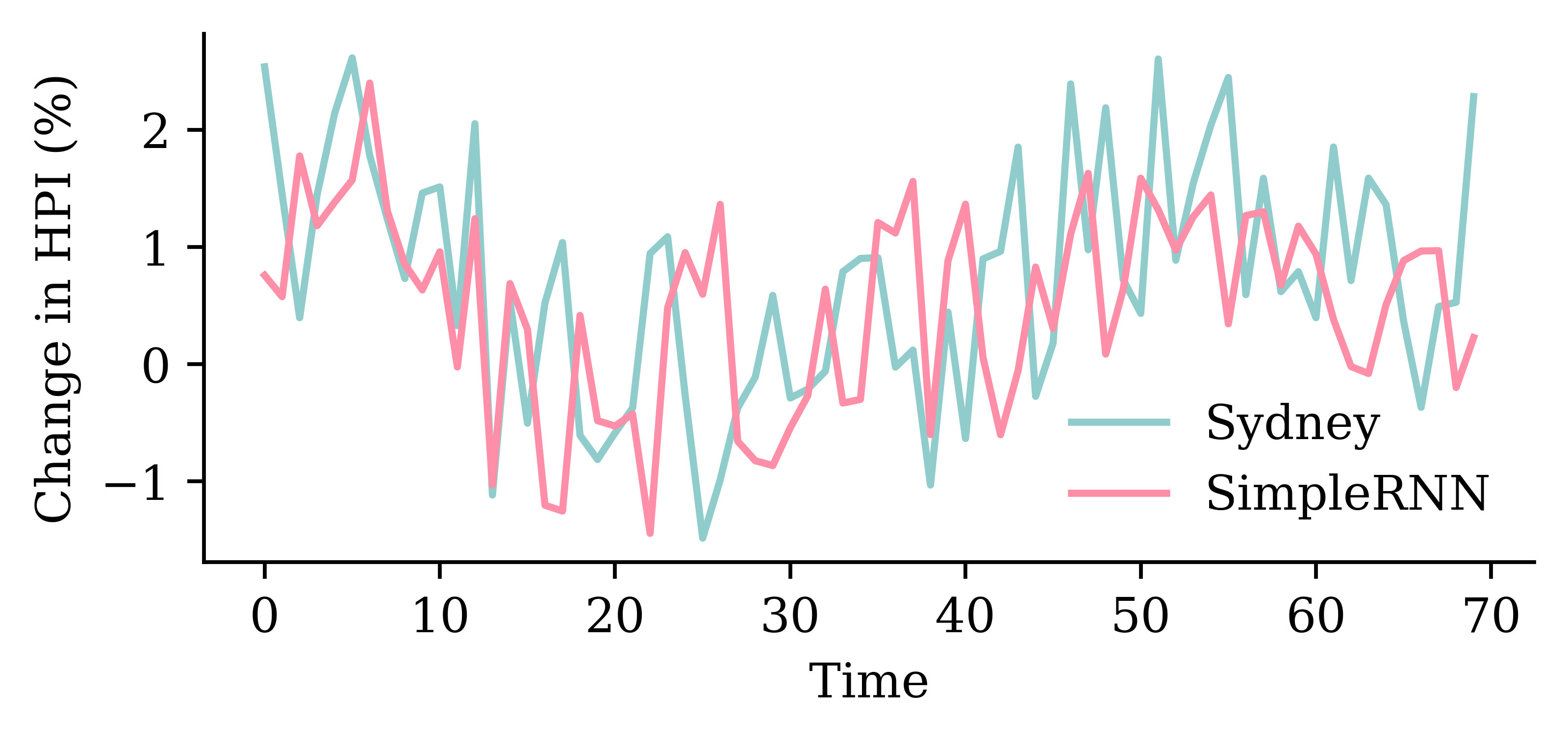
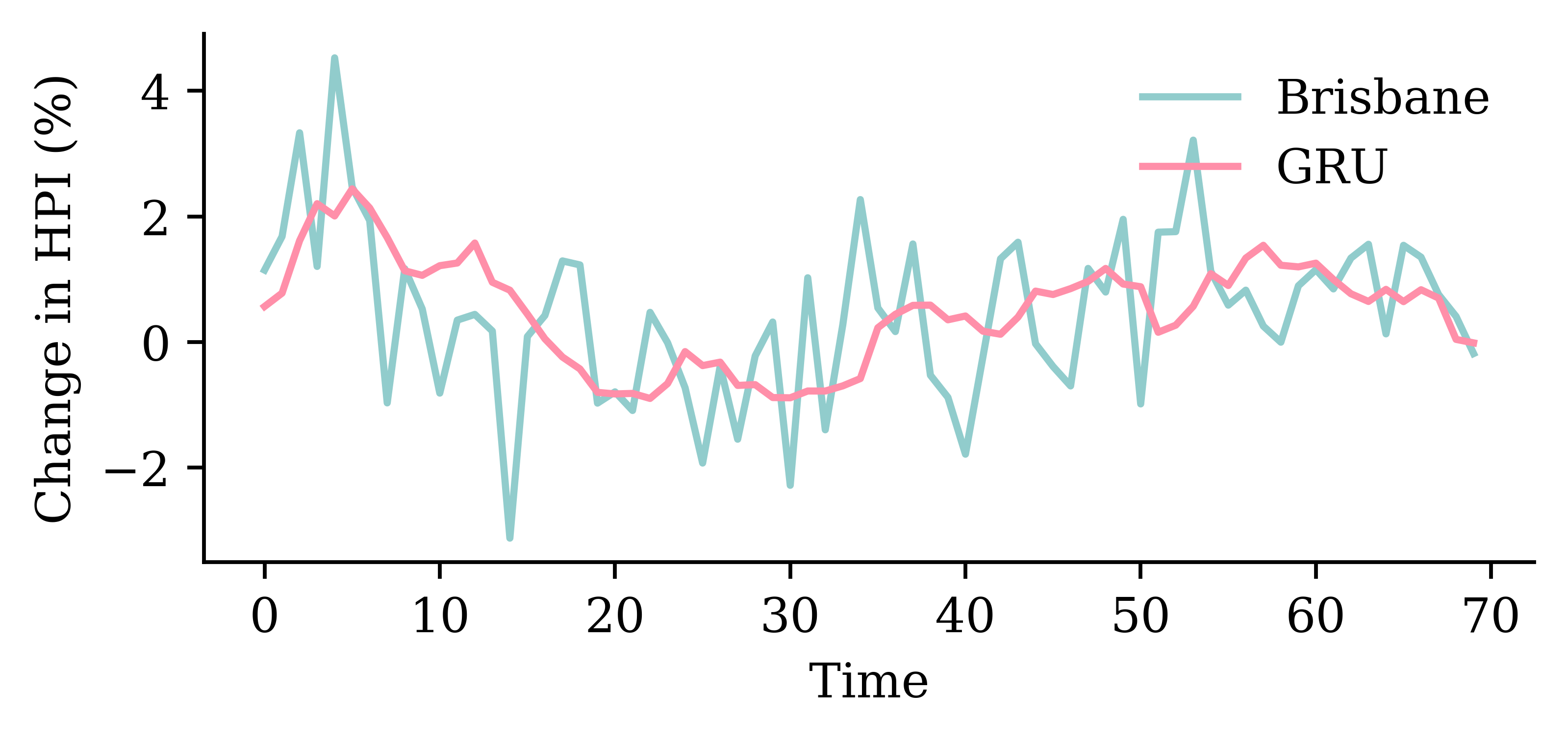
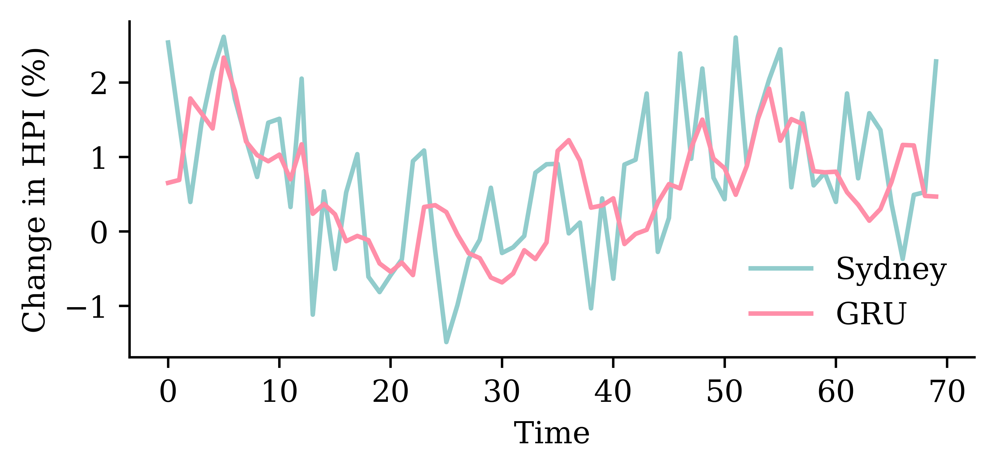
target_suburb = changes["Sydney"]

train_ds = \
  timeseries_dataset_from_array(
    changes[:-delay],
    targets=target_suburb[delay:],
    sequence_length=seq_length,
    end_index=num_train)

val_ds = \
  timeseries_dataset_from_array(
    changes[:-delay],
    targets=target_suburb[delay:],
    sequence_length=seq_length,
    start_index=num_train,
    end_index=num_train+num_val)

test_ds = \
  timeseries_dataset_from_array(
    changes[:-delay],
    targets=target_suburb[delay:],
    sequence_length=seq_length,
    start_index=num_train+num_val)

Converting `Dataset` to numpy

The Dataset object can be handed to Keras directly, but if we really need a numpy array, we can run:

X_train = np.concatenate(list(train_ds.map(lambda x, y: x)))
y_train = np.concatenate(list(train_ds.map(lambda x, y: y)))

The shape of our training set is now:

X_train.shape

(220, 6, 7)

y_train.shape

(220,)

Later, we need the targets as numpy arrays:

y_train = np.concatenate(list(train_ds.map(lambda x, y: y)))
y_val = np.concatenate(list(val_ds.map(lambda x, y: y)))
y_test = np.concatenate(list(test_ds.map(lambda x, y: y)))

A dense network

from keras.layers import Input, Flatten
random.seed(1)
model_dense = Sequential([
    Input((seq_length, num_ts)),
    Flatten(),
    Dense(50, activation="leaky_relu"),
    Dense(20, activation="leaky_relu"),
    Dense(1, activation="linear")
])
model_dense.compile(loss="mse", optimizer="adam")
print(f"This model has {model_dense.count_params()} parameters.")

es = EarlyStopping(patience=50, restore_best_weights=True, verbose=1)
%time hist = model_dense.fit(train_ds, epochs=1_000, \
  validation_data=val_ds, callbacks=[es], verbose=0);

This model has 3191 parameters.
Epoch 126: early stopping
Restoring model weights from the end of the best epoch: 76.
CPU times: user 6.48 s, sys: 3.55 s, total: 10 s
Wall time: 3.4 s

Plot the model

from keras.utils import plot_model
plot_model(model_dense, show_shapes=True)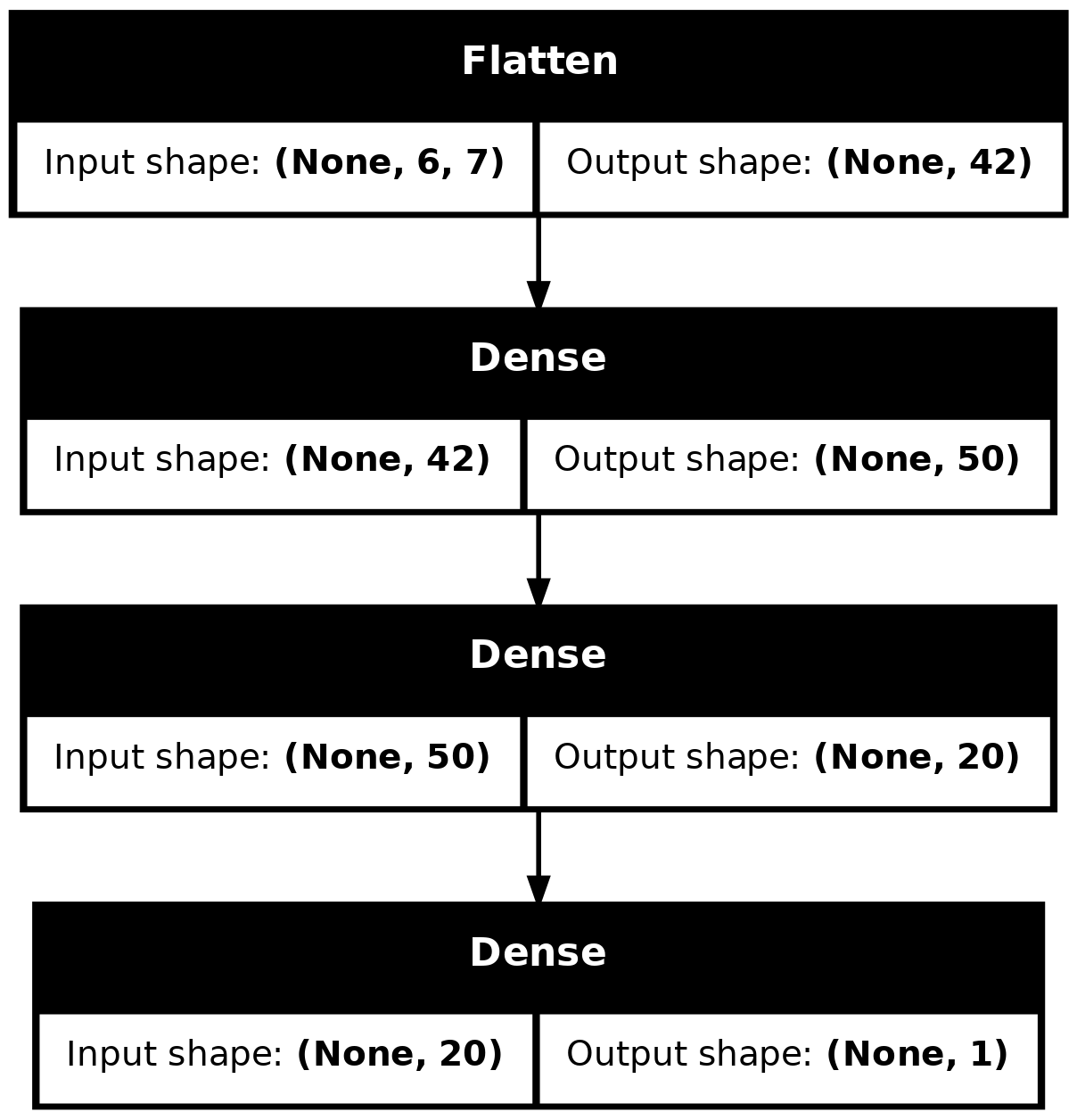

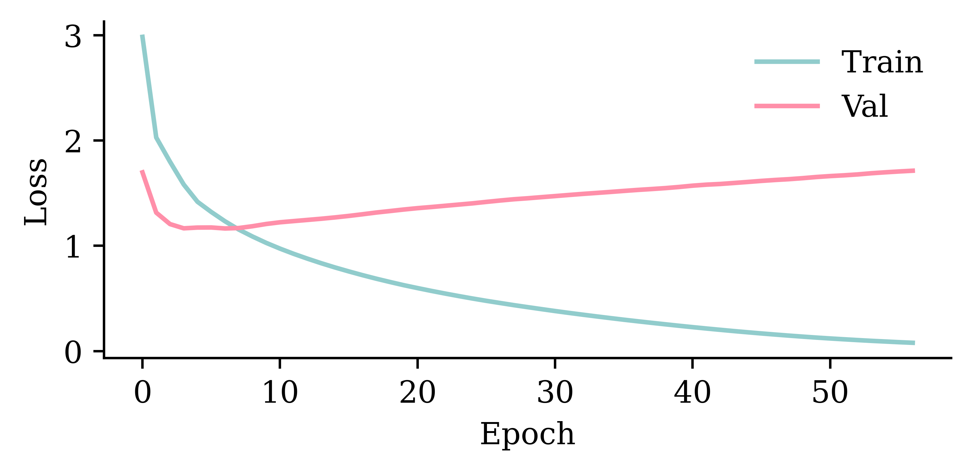
Assess the fits

model_dense.evaluate(val_ds, verbose=0)

1.3521653413772583

Plotting the predictions

A `SimpleRNN` layer

random.seed(1)

model_simple = Sequential([
    Input((seq_length, num_ts)),
    SimpleRNN(50),
    Dense(1, activation="linear")
])
model_simple.compile(loss="mse", optimizer="adam")
print(f"This model has {model_simple.count_params()} parameters.")

es = EarlyStopping(patience=50, restore_best_weights=True, verbose=1)
%time hist = model_simple.fit(train_ds, epochs=1_000, \
  validation_data=val_ds, callbacks=[es], verbose=0);

This model has 2951 parameters.
Epoch 57: early stopping
Restoring model weights from the end of the best epoch: 7.
CPU times: user 3.07 s, sys: 1.54 s, total: 4.61 s
Wall time: 1.71 s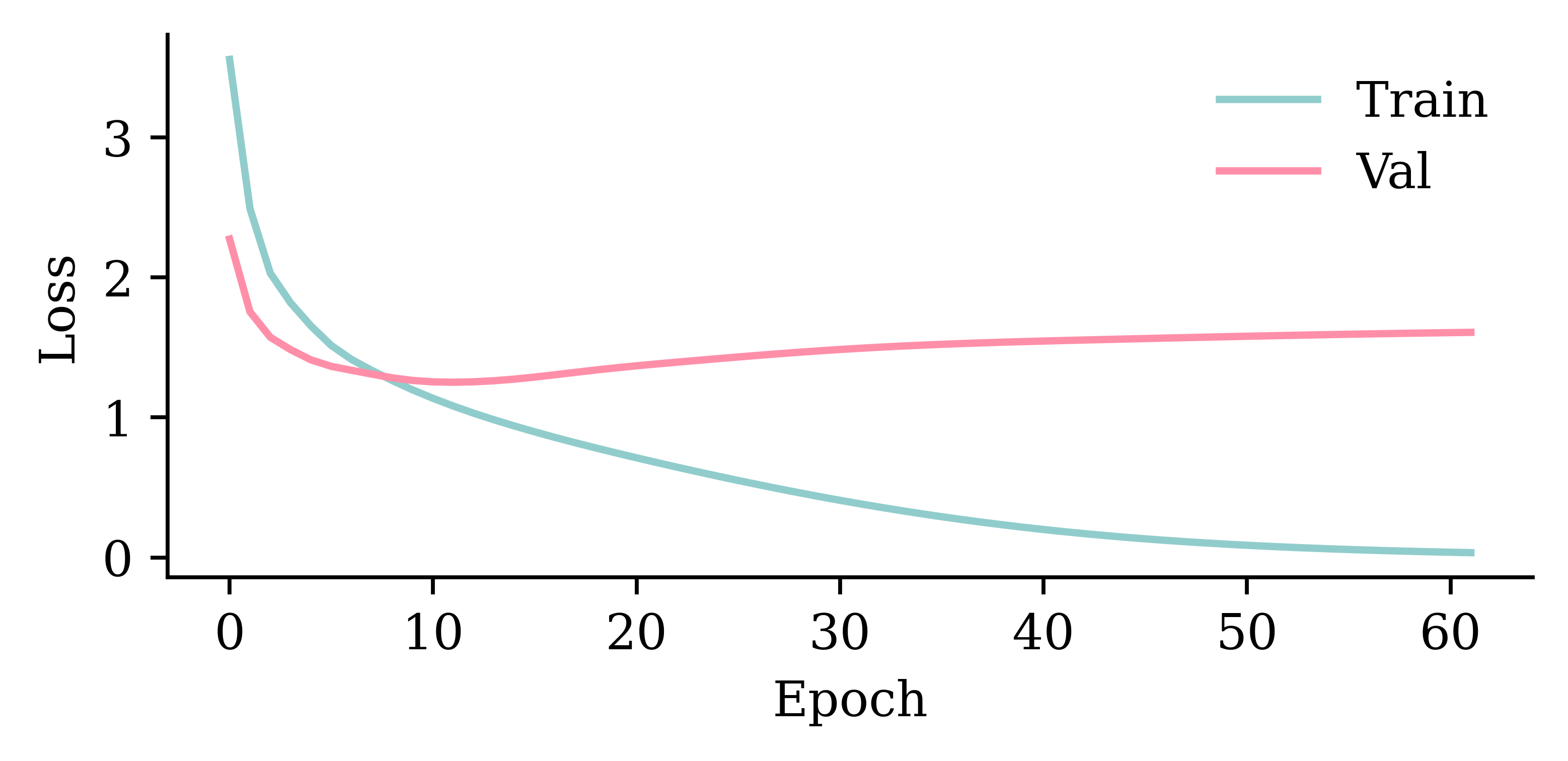

Assess the fits

model_simple.evaluate(val_ds, verbose=0)

0.8697079420089722

Plot the model

plot_model(model_simple, show_shapes=True)

Plotting the predictions

A `LSTM` layer

from keras.layers import LSTM

random.seed(1)

model_lstm = Sequential([
    Input((seq_length, num_ts)),
    LSTM(50),
    Dense(1, activation="linear")
])

model_lstm.compile(loss="mse", optimizer="adam")

es = EarlyStopping(patience=50, restore_best_weights=True, verbose=1)

%time hist = model_lstm.fit(train_ds, epochs=1_000, \
  validation_data=val_ds, callbacks=[es], verbose=0);

Epoch 72: early stopping
Restoring model weights from the end of the best epoch: 22.
CPU times: user 4.09 s, sys: 2 s, total: 6.09 s
Wall time: 2.39 s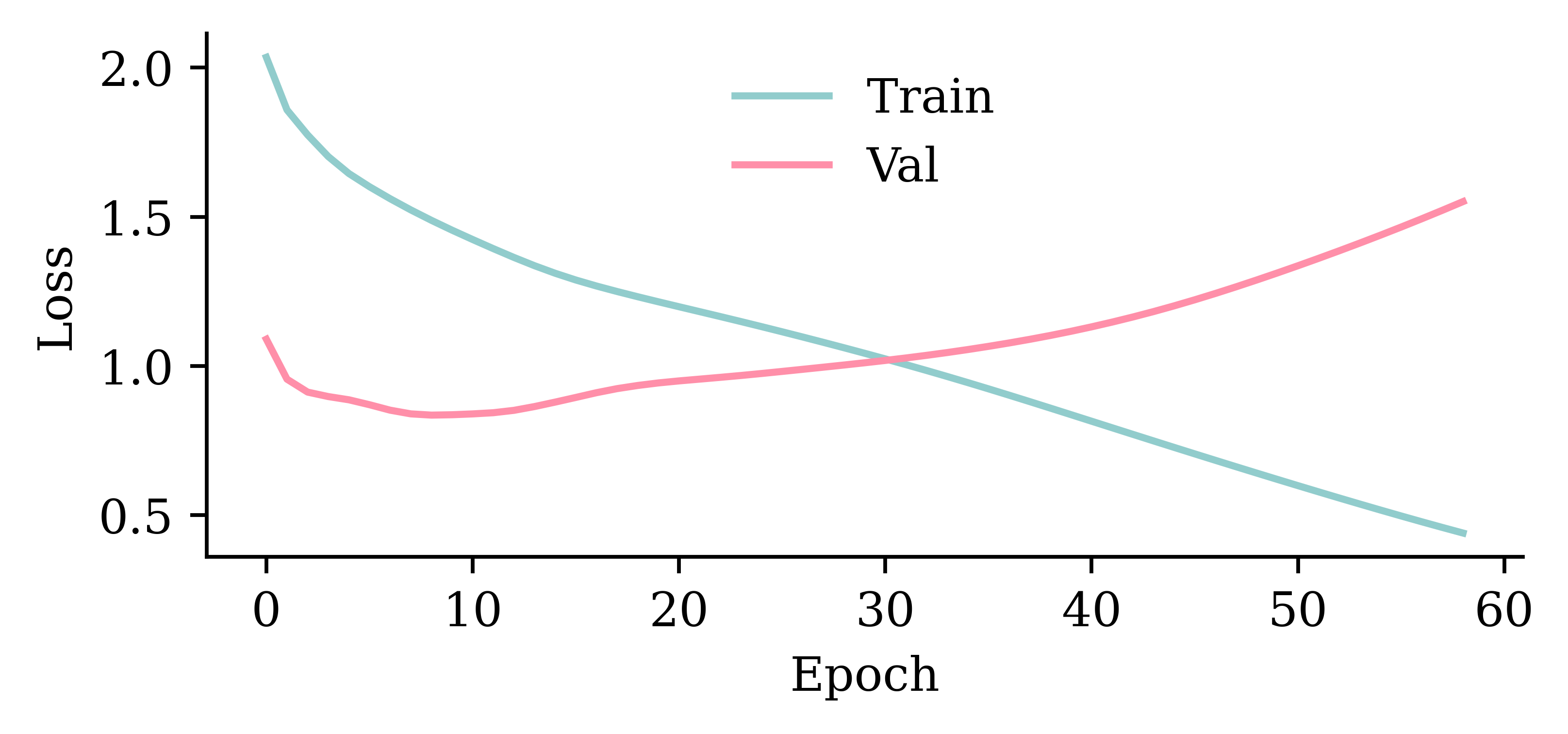

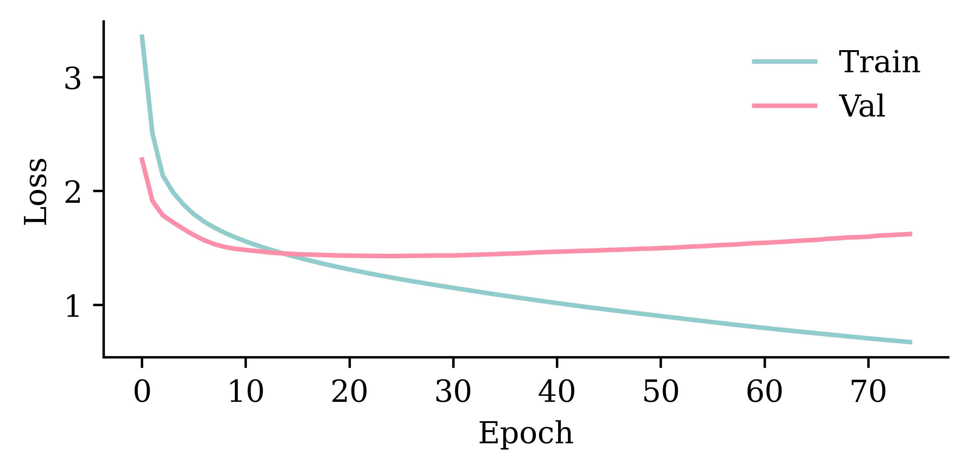
Assess the fits

model_lstm.evaluate(val_ds, verbose=0)

0.8331283330917358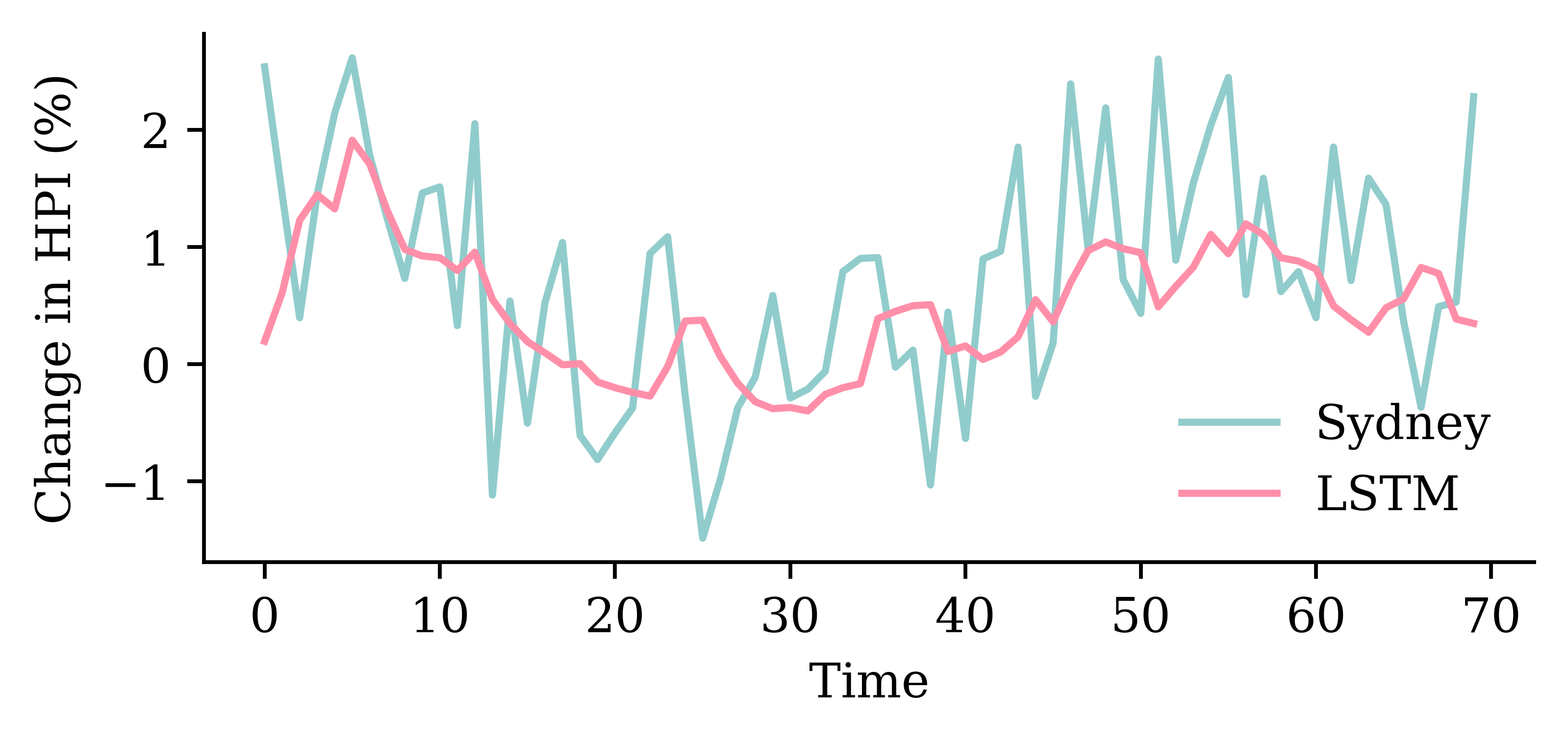

Plotting the predictions

A `GRU` layer

from keras.layers import GRU

random.seed(1)

model_gru = Sequential([
    Input((seq_length, num_ts)),
    GRU(50),
    Dense(1, activation="linear")
])

model_gru.compile(loss="mse", optimizer="adam")

es = EarlyStopping(patience=50, restore_best_weights=True, verbose=1)

%time hist = model_gru.fit(train_ds, epochs=1_000, \
  validation_data=val_ds, callbacks=[es], verbose=0)

Epoch 66: early stopping
Restoring model weights from the end of the best epoch: 16.
CPU times: user 3.81 s, sys: 1.82 s, total: 5.63 s
Wall time: 2.21 s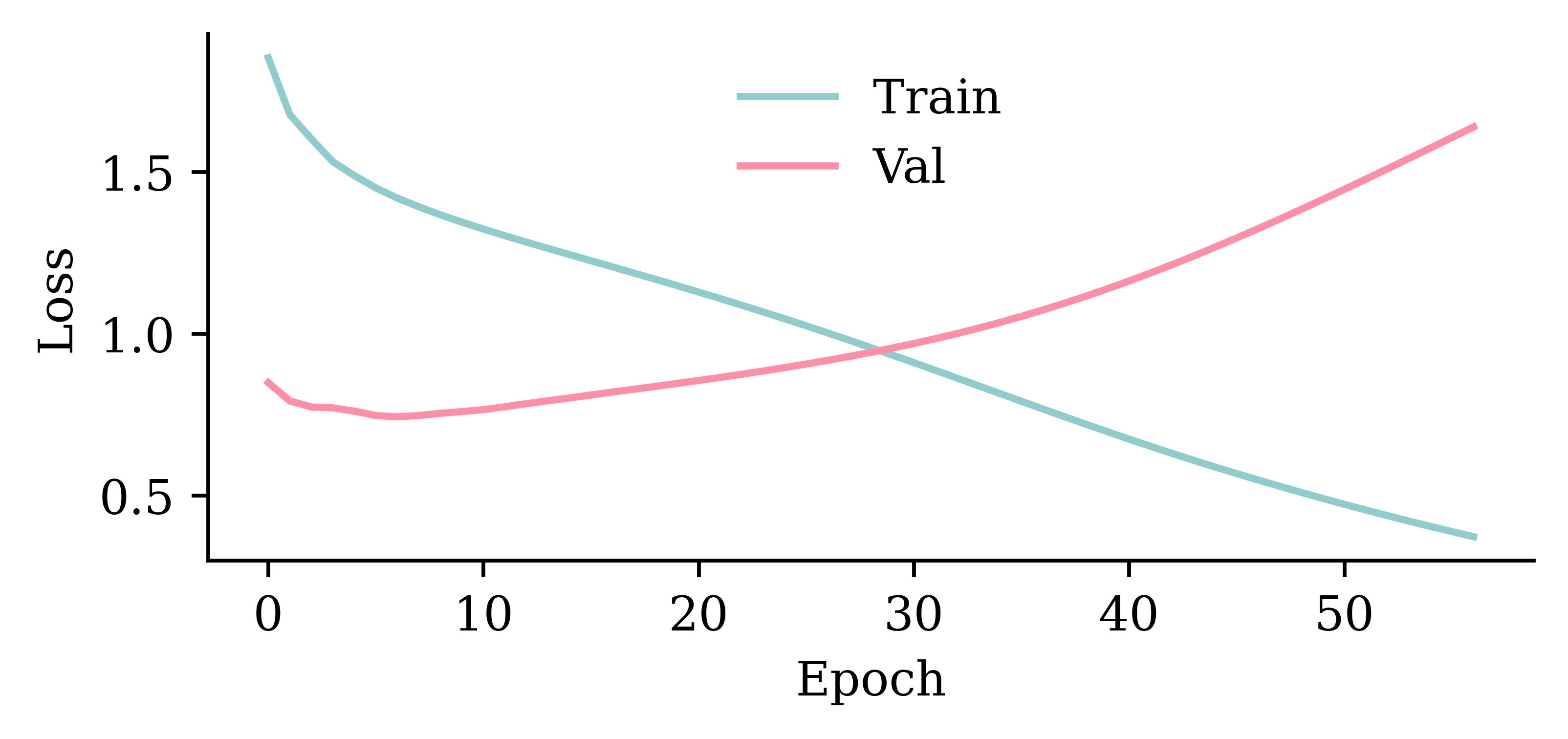

Assess the fits

model_gru.evaluate(val_ds, verbose=0)

0.8188608884811401

Plotting the predictions

Two `GRU` layers

random.seed(1)

model_two_grus = Sequential([
    Input((seq_length, num_ts)),
    GRU(50, return_sequences=True),
    GRU(50),
    Dense(1, activation="linear")
])

model_two_grus.compile(loss="mse", optimizer="adam")

es = EarlyStopping(patience=50, restore_best_weights=True, verbose=1)

%time hist = model_two_grus.fit(train_ds, epochs=1_000, \
  validation_data=val_ds, callbacks=[es], verbose=0)

Epoch 69: early stopping
Restoring model weights from the end of the best epoch: 19.
CPU times: user 4.5 s, sys: 1.93 s, total: 6.43 s
Wall time: 2.88 s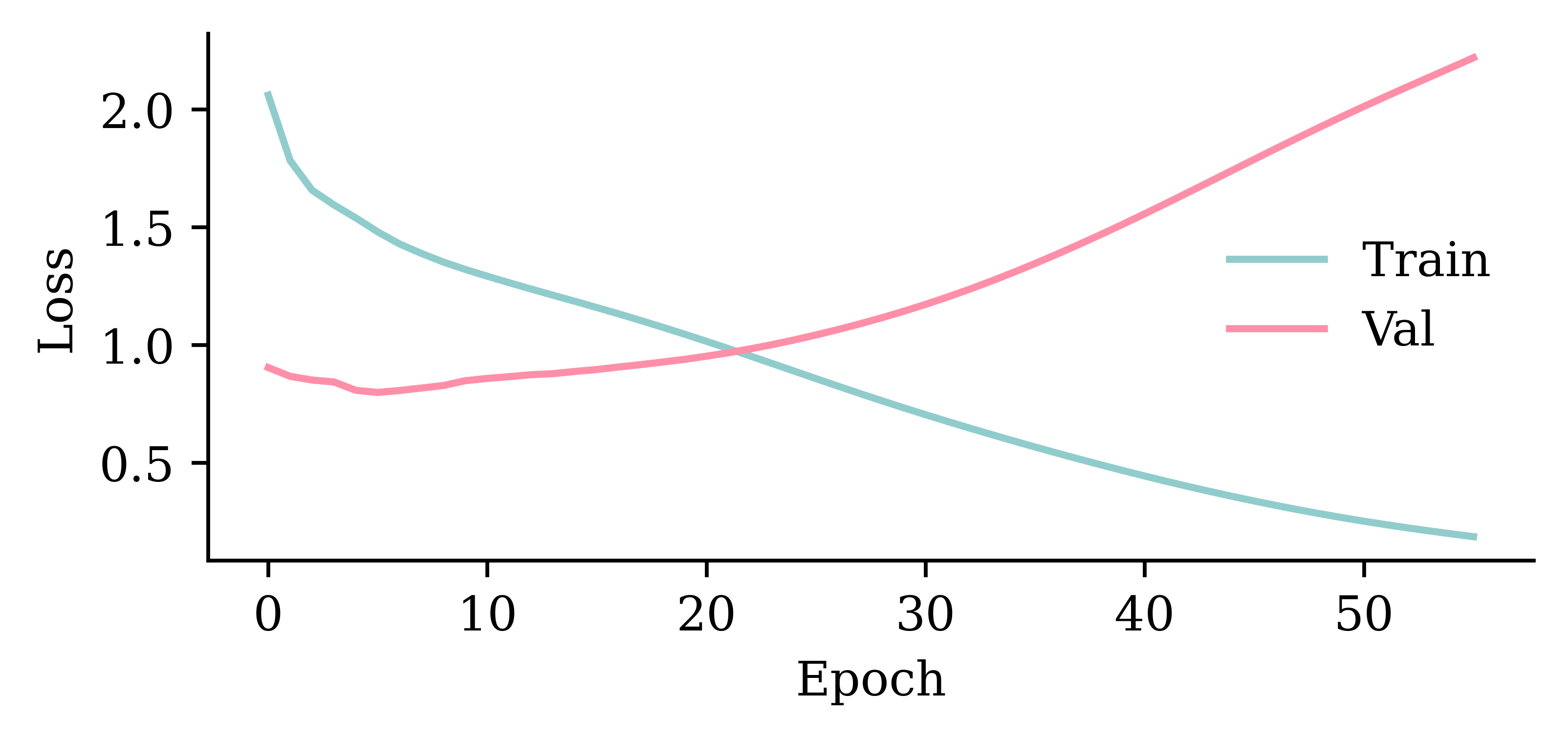

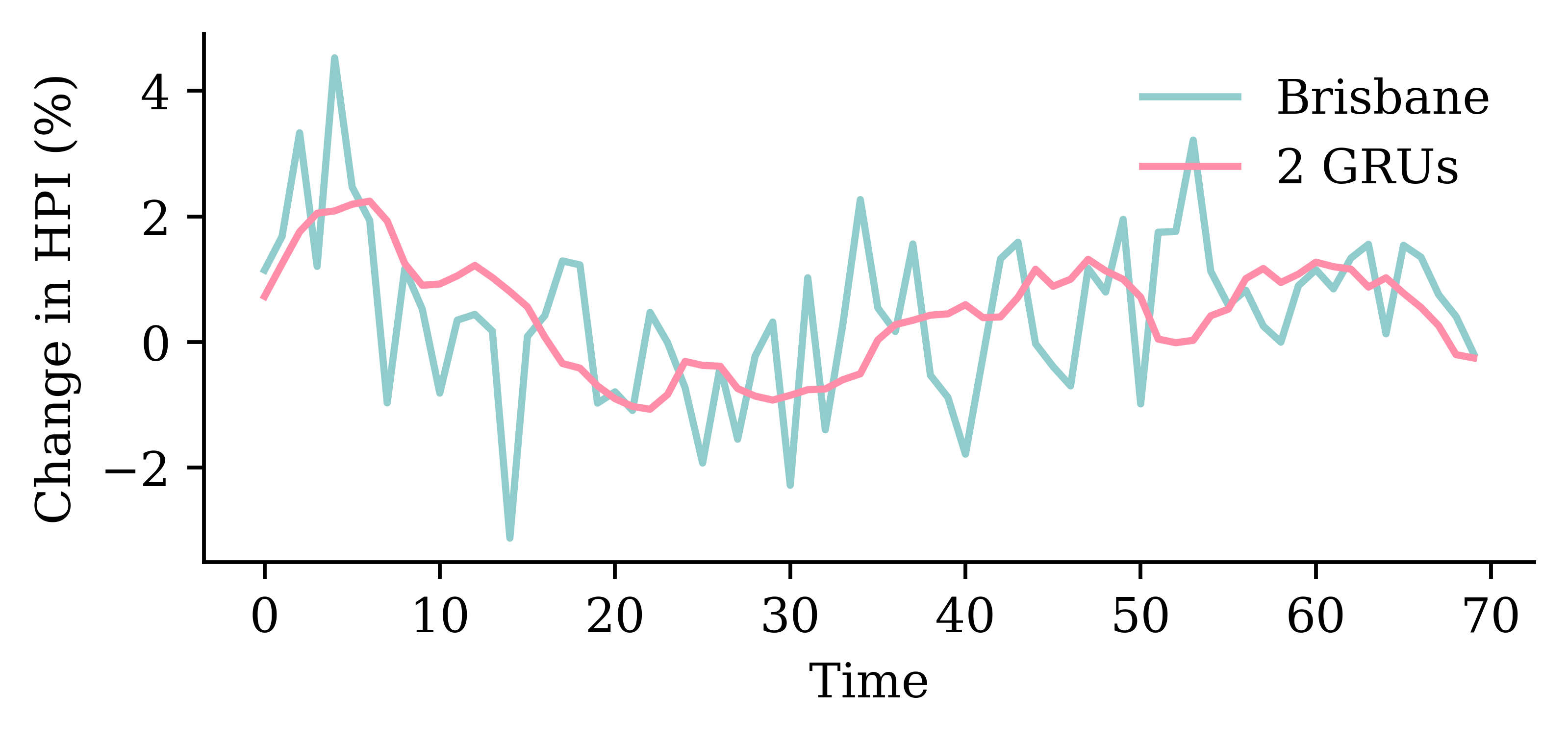
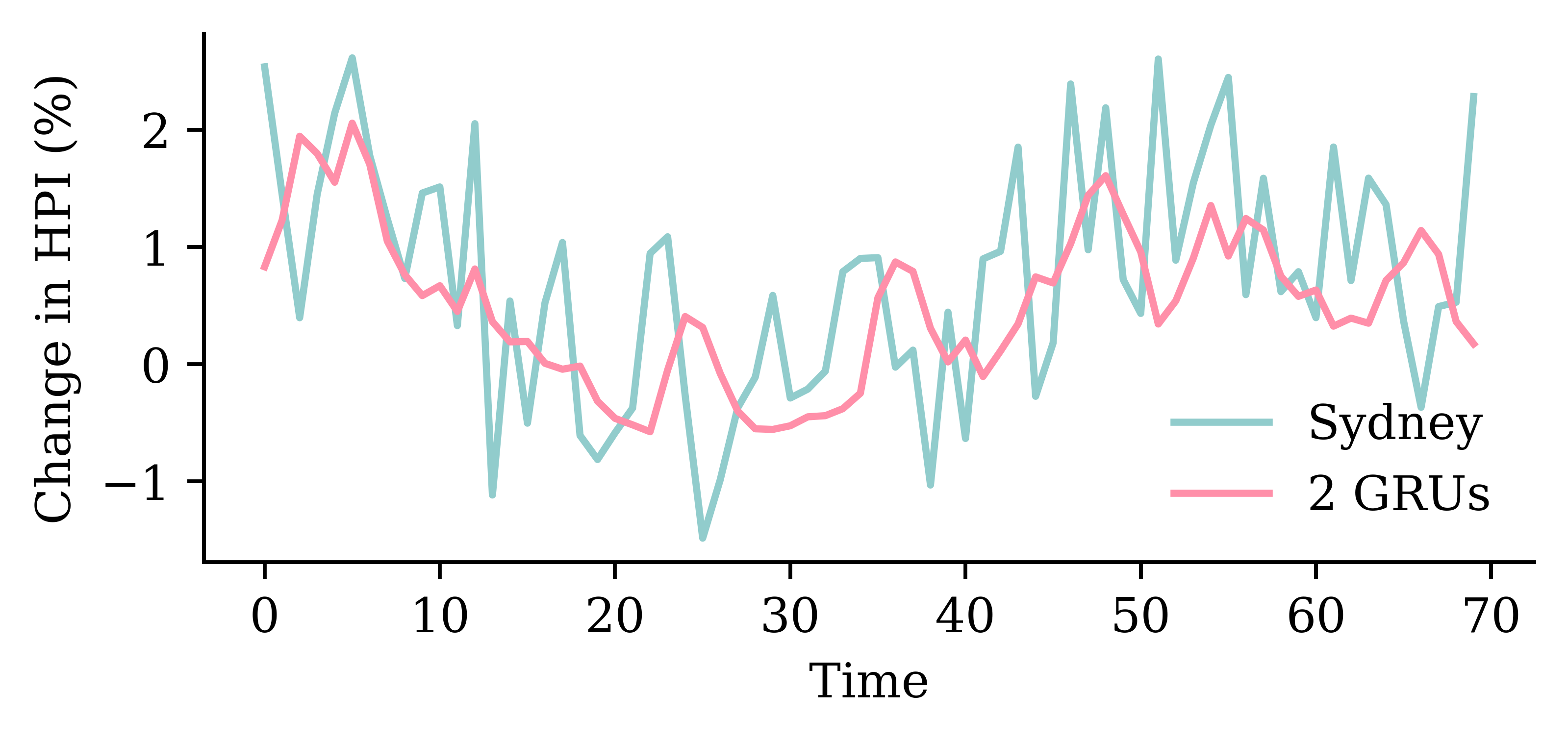
Assess the fits

model_two_grus.evaluate(val_ds, verbose=0)

0.777770459651947

Plotting the predictions

Compare the models

	Model	MSE
0	Dense	1.352165
1	SimpleRNN	0.869708
2	LSTM	0.833128
3	GRU	0.818861
4	2 GRUs	0.777770

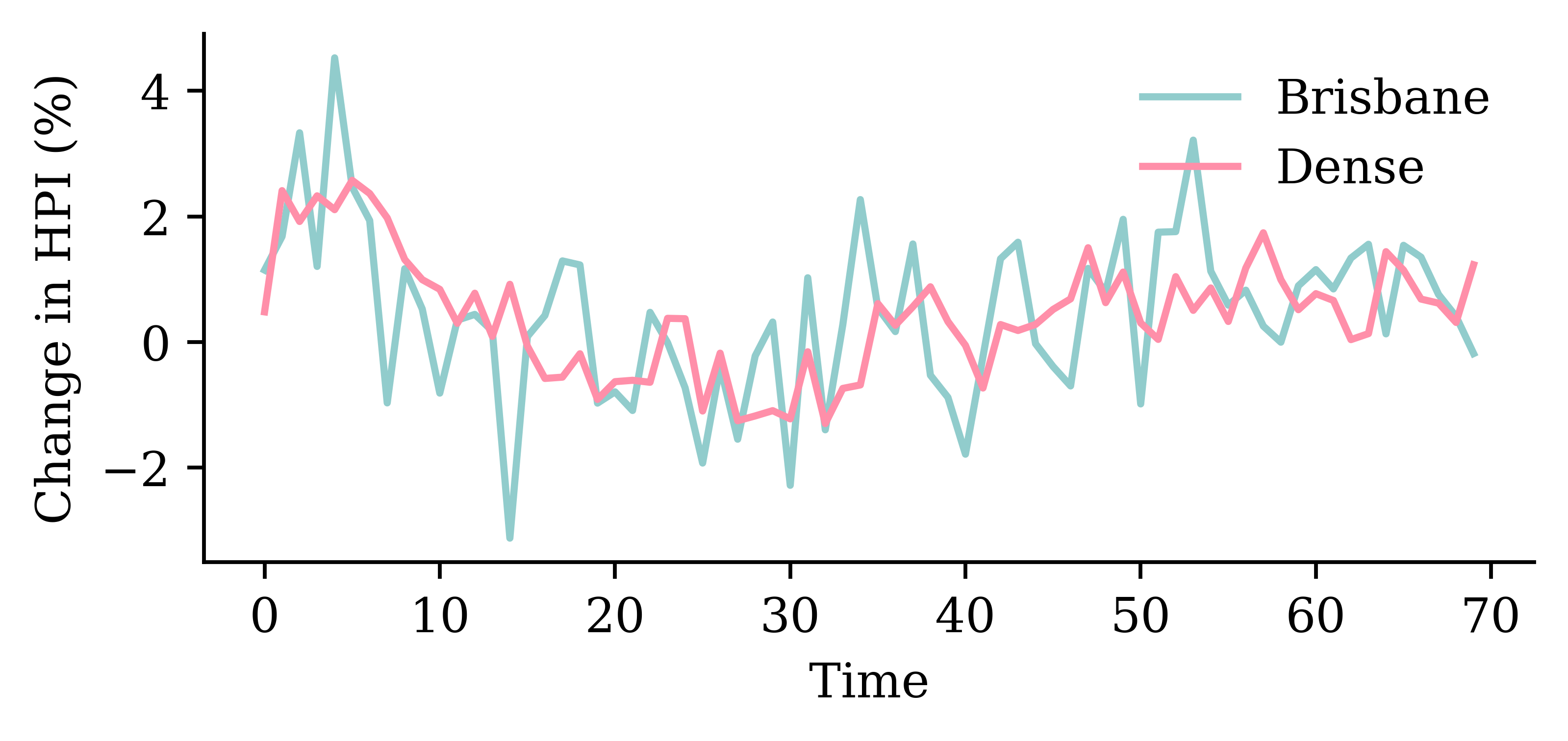
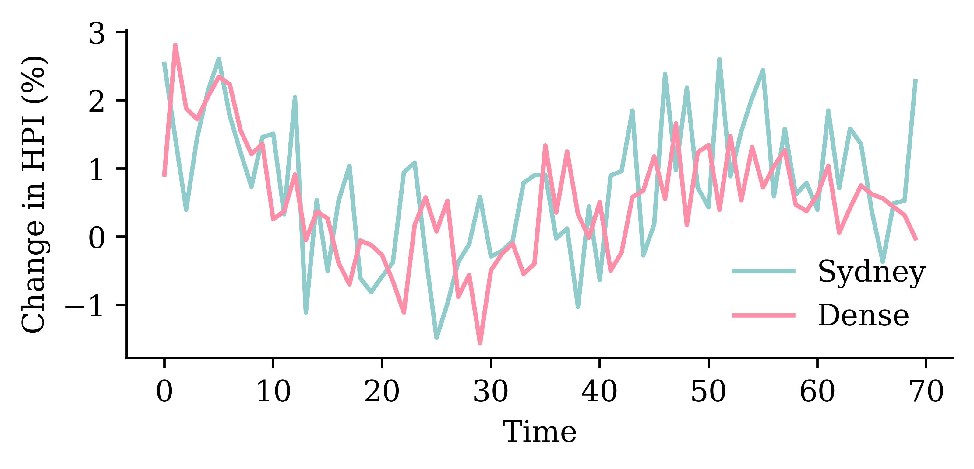
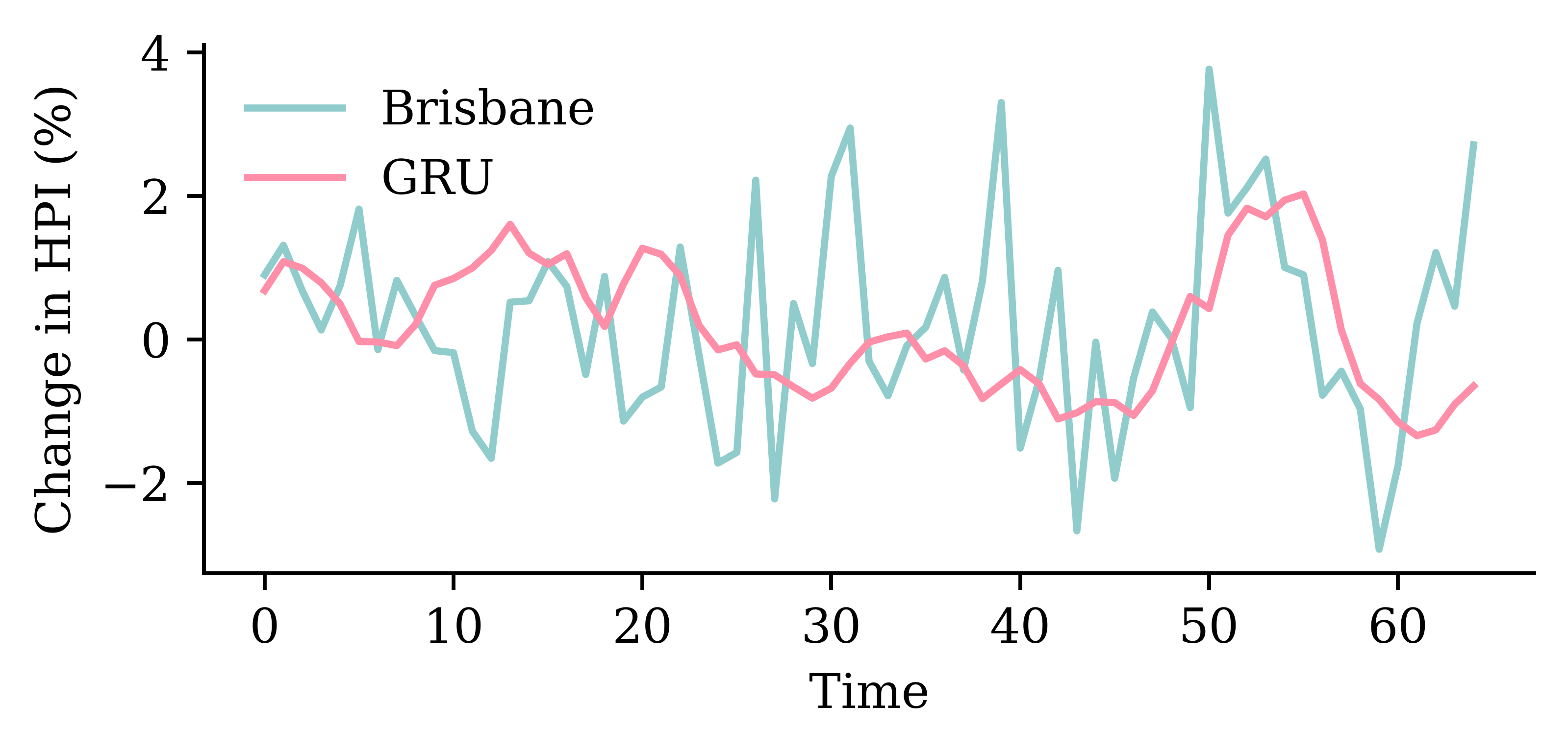
The network with two GRU layers is the best.

model_two_grus.evaluate(test_ds, verbose=0)

1.9774343967437744

Test set

Predicting Multiple Time Series

Creating dataset objects

Change the targets argument to include all the suburbs.

train_ds = \
  timeseries_dataset_from_array(
    changes[:-delay],
    targets=changes[delay:],
    sequence_length=seq_length,
    end_index=num_train)

val_ds = \
  timeseries_dataset_from_array(
    changes[:-delay],
    targets=changes[delay:],
    sequence_length=seq_length,
    start_index=num_train,
    end_index=num_train+num_val)

test_ds = \
  timeseries_dataset_from_array(
    changes[:-delay],
    targets=changes[delay:],
    sequence_length=seq_length,
    start_index=num_train+num_val)

Converting `Dataset` to numpy

The shape of our training set is now:

X_train = np.concatenate(list(train_ds.map(lambda x, y: x)))
X_train.shape

(220, 6, 7)

Y_train = np.concatenate(list(train_ds.map(lambda x, y: y)))
Y_train.shape

(220, 7)

Later, we need the targets as numpy arrays:

Y_train = np.concatenate(list(train_ds.map(lambda x, y: y)))
Y_val = np.concatenate(list(val_ds.map(lambda x, y: y)))
Y_test = np.concatenate(list(test_ds.map(lambda x, y: y)))

A dense network

random.seed(1)
model_dense = Sequential([
    Input((seq_length, num_ts)),
    Flatten(),
    Dense(50, activation="leaky_relu"),
    Dense(20, activation="leaky_relu"),
    Dense(num_ts, activation="linear")
])
model_dense.compile(loss="mse", optimizer="adam")
print(f"This model has {model_dense.count_params()} parameters.")

es = EarlyStopping(patience=50, restore_best_weights=True, verbose=1)
%time hist = model_dense.fit(train_ds, epochs=1_000, \
  validation_data=val_ds, callbacks=[es], verbose=0);

This model has 3317 parameters.
Epoch 96: early stopping
Restoring model weights from the end of the best epoch: 46.
CPU times: user 4.97 s, sys: 2.69 s, total: 7.66 s
Wall time: 2.65 s

Plot the model

plot_model(model_dense, show_shapes=True)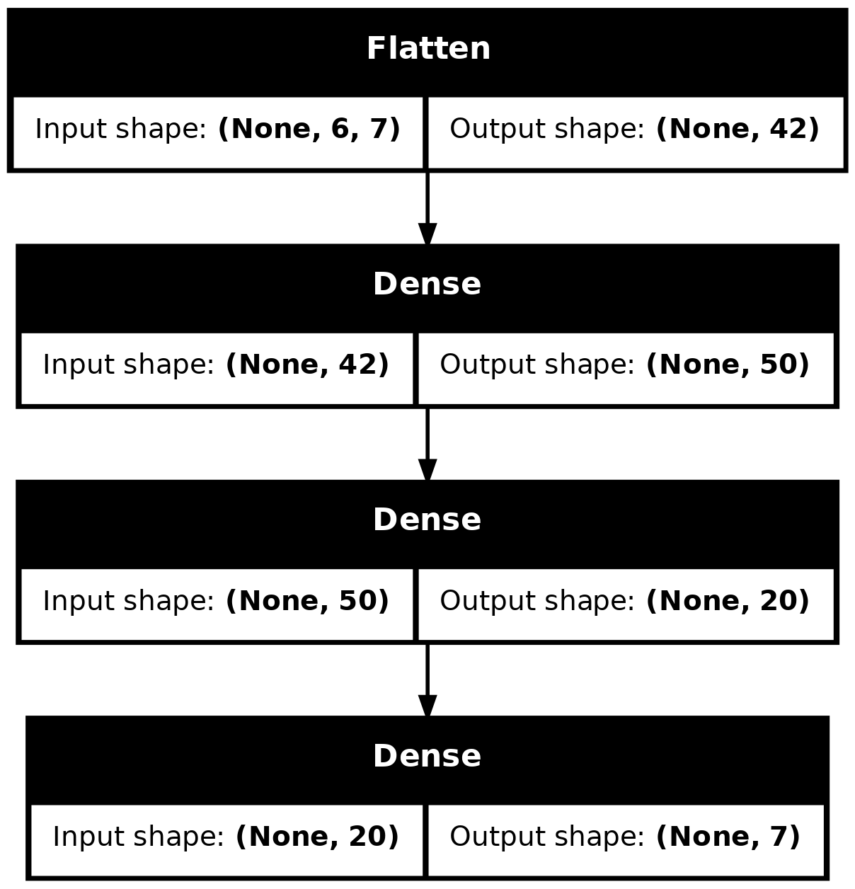

Assess the fits

model_dense.evaluate(val_ds, verbose=0)

1.445832371711731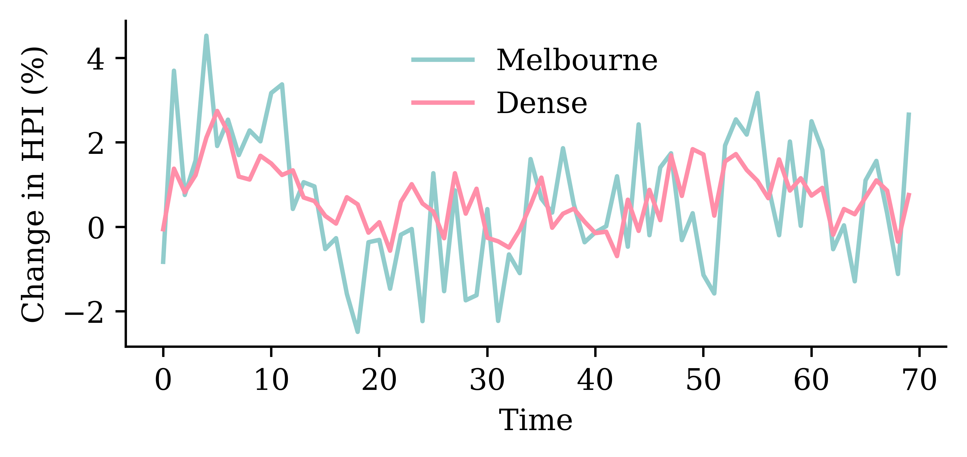

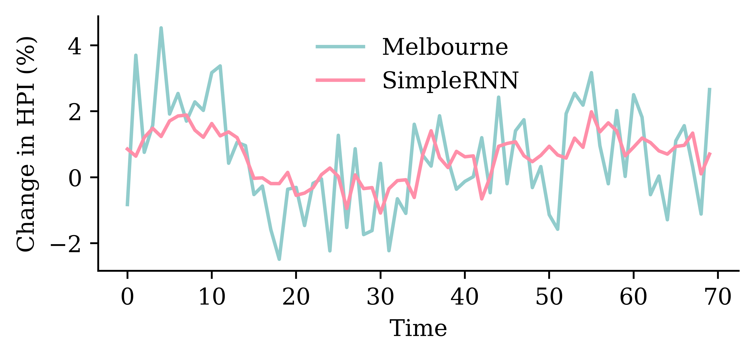
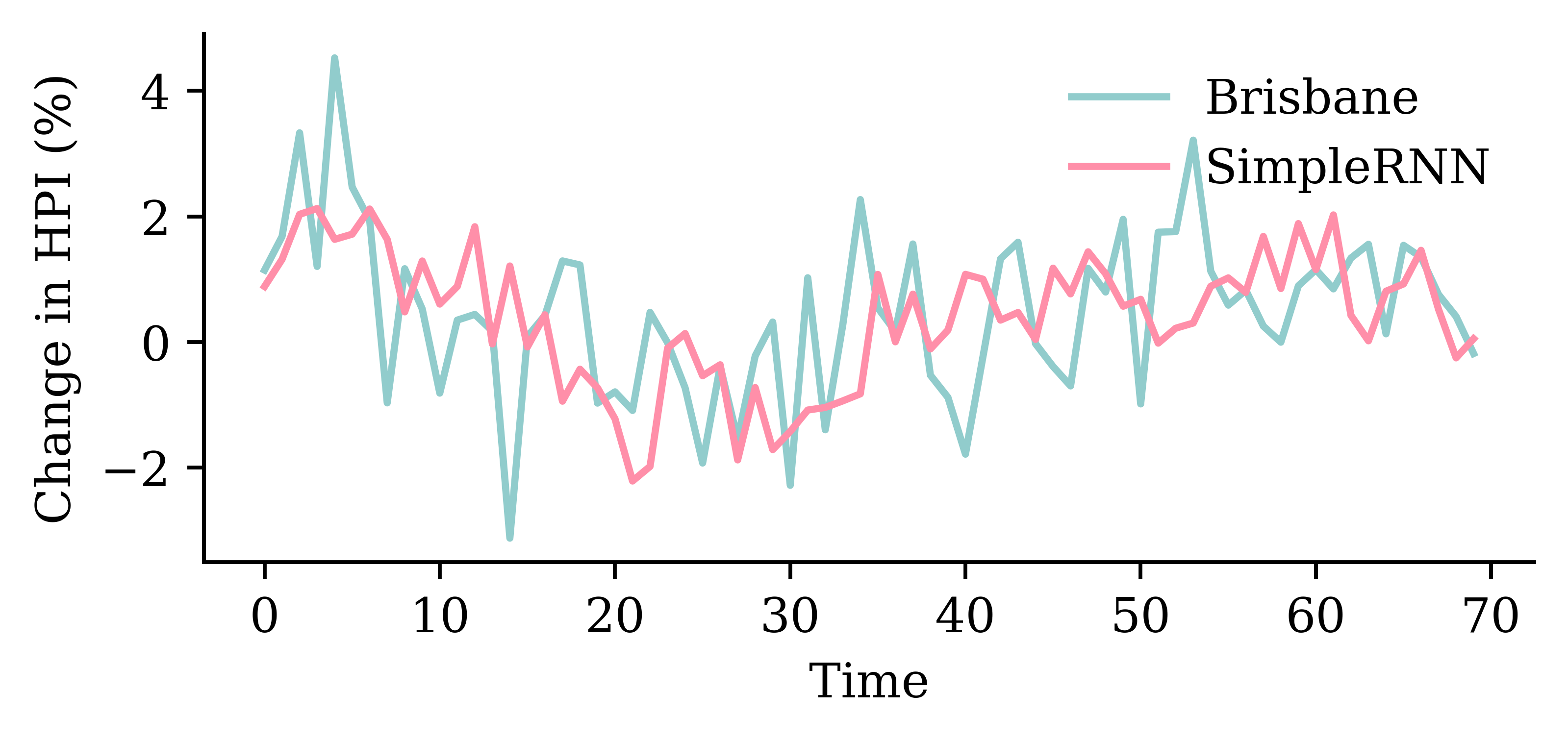
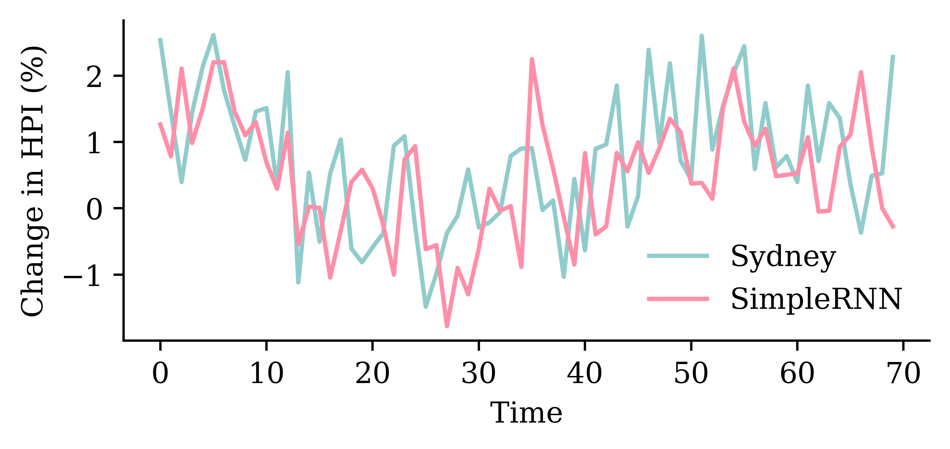
Plotting the predictions

A `SimpleRNN` layer

random.seed(1)

model_simple = Sequential([
    Input((seq_length, num_ts)),
    SimpleRNN(50),
    Dense(num_ts, activation="linear")
])
model_simple.compile(loss="mse", optimizer="adam")
print(f"This model has {model_simple.count_params()} parameters.")

es = EarlyStopping(patience=50, restore_best_weights=True, verbose=1)
%time hist = model_simple.fit(train_ds, epochs=1_000, \
  validation_data=val_ds, callbacks=[es], verbose=0);

This model has 3257 parameters.
Epoch 93: early stopping
Restoring model weights from the end of the best epoch: 43.
CPU times: user 5.08 s, sys: 2.59 s, total: 7.67 s
Wall time: 2.82 s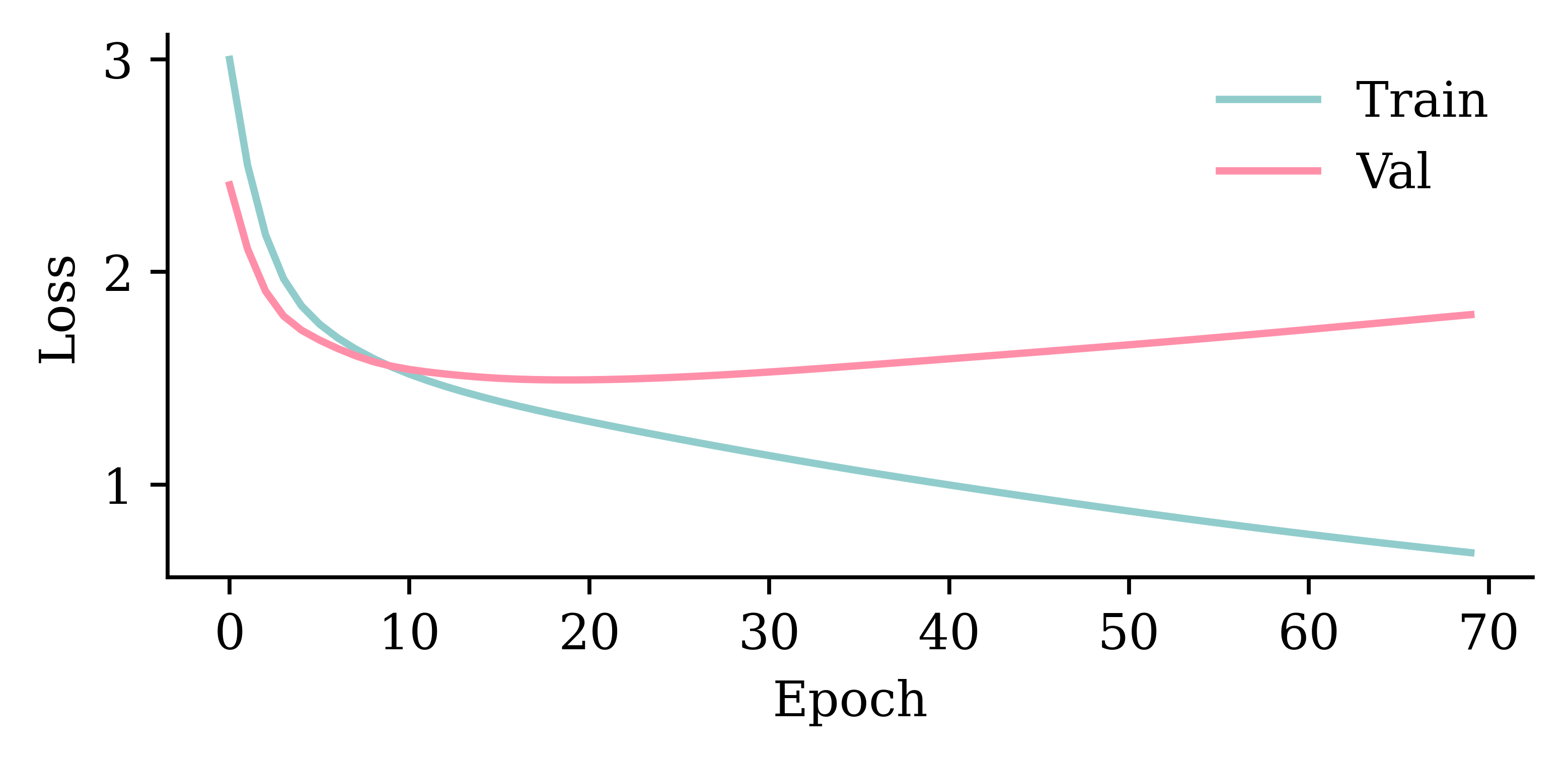

Assess the fits

model_simple.evaluate(val_ds, verbose=0)

1.6287589073181152

Plot the model

plot_model(model_simple, show_shapes=True)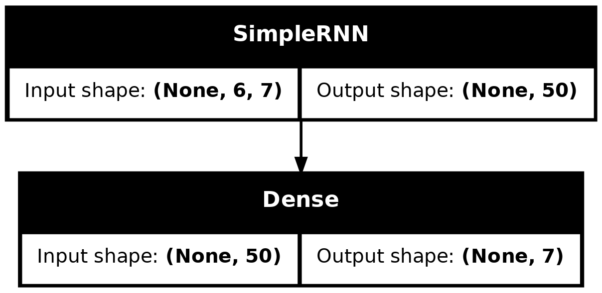

Plotting the predictions

A `LSTM` layer

random.seed(1)

model_lstm = Sequential([
    Input((seq_length, num_ts)),
    LSTM(50),
    Dense(num_ts, activation="linear")
])

model_lstm.compile(loss="mse", optimizer="adam")

es = EarlyStopping(patience=50, restore_best_weights=True, verbose=1)

%time hist = model_lstm.fit(train_ds, epochs=1_000, \
  validation_data=val_ds, callbacks=[es], verbose=0);

Epoch 106: early stopping
Restoring model weights from the end of the best epoch: 56.
CPU times: user 6.13 s, sys: 3.03 s, total: 9.16 s
Wall time: 3.56 s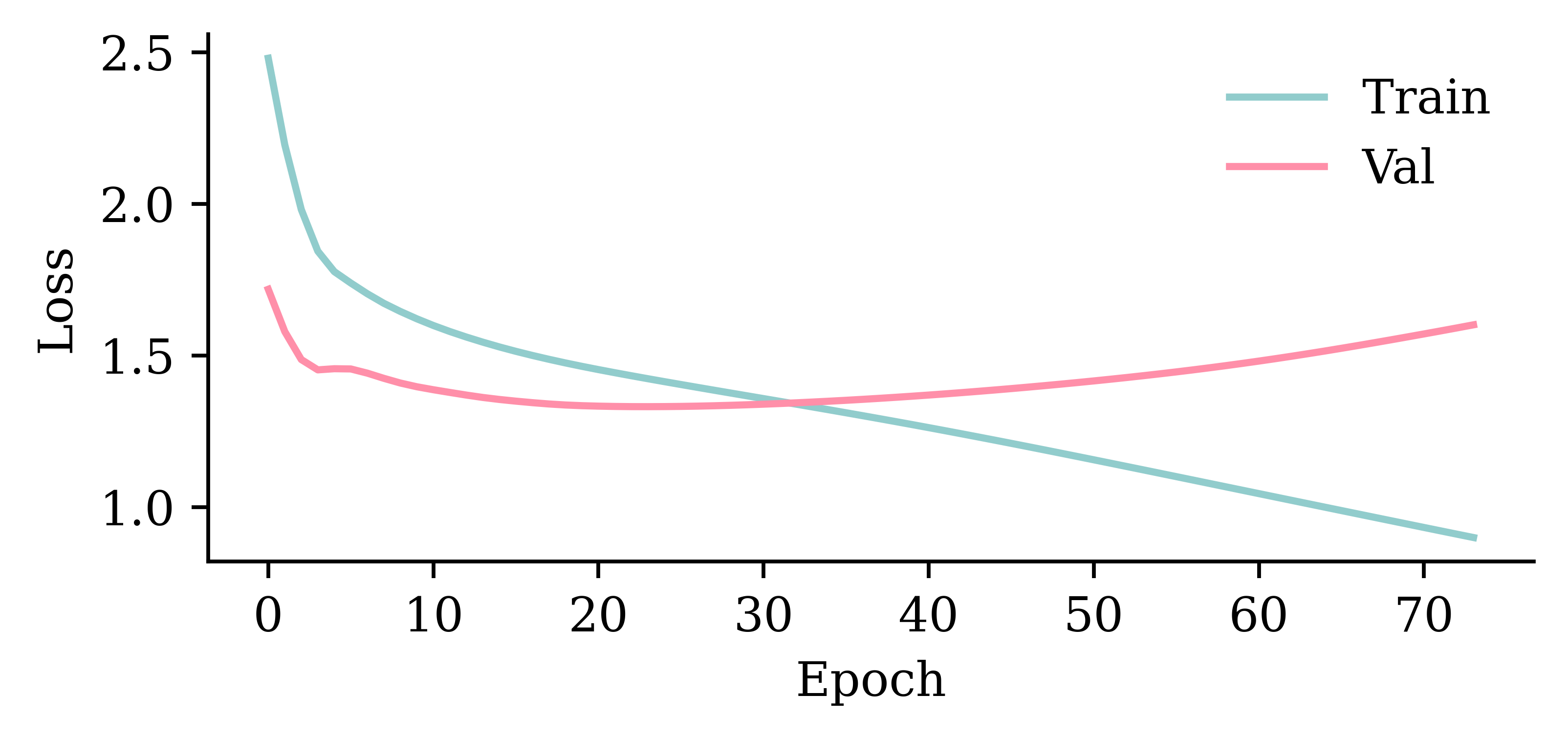

Assess the fits

model_lstm.evaluate(val_ds, verbose=0)

1.3439931869506836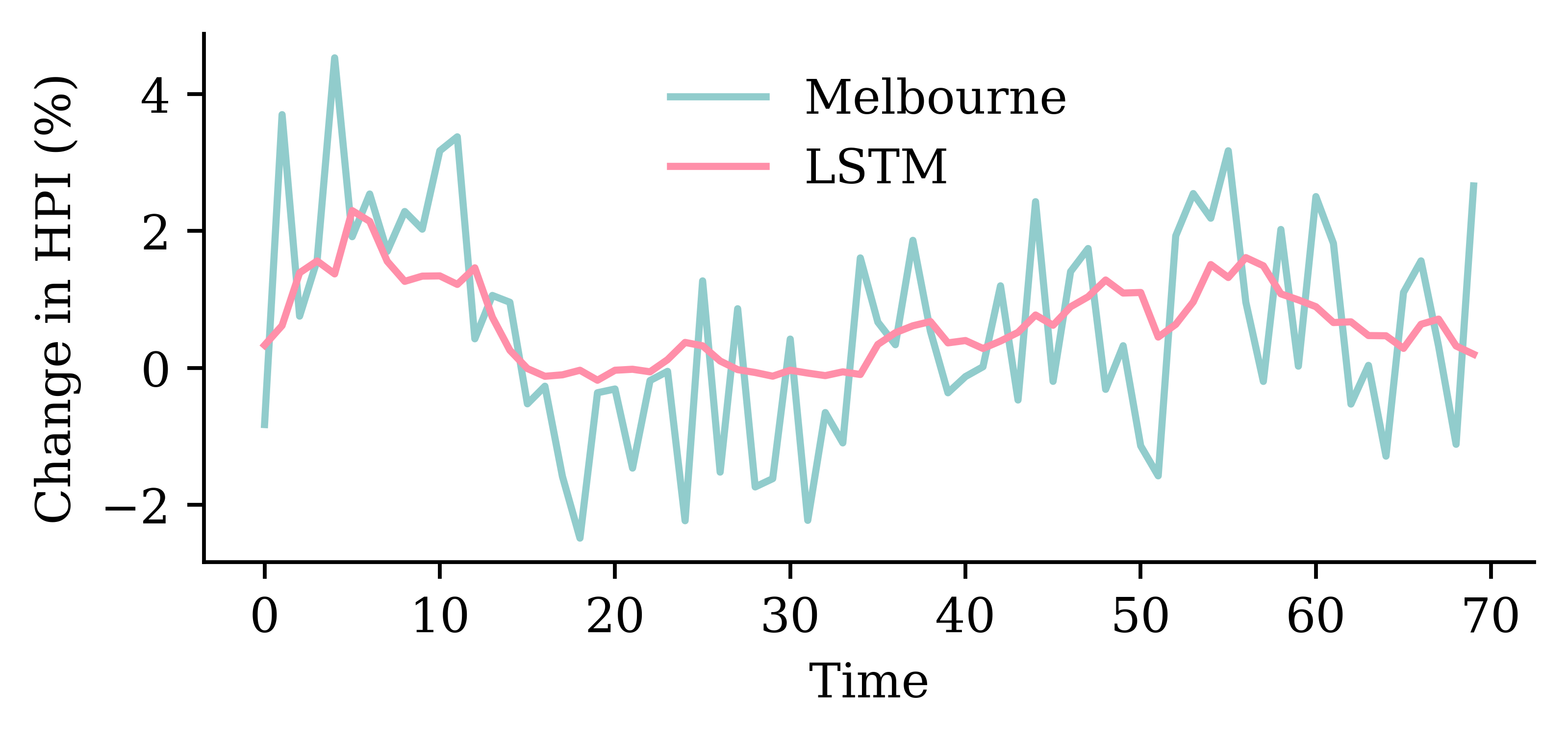

Plotting the predictions

A `GRU` layer

random.seed(1)

model_gru = Sequential([
    Input((seq_length, num_ts)),
    GRU(50),
    Dense(num_ts, activation="linear")
])

model_gru.compile(loss="mse", optimizer="adam")

es = EarlyStopping(patience=50, restore_best_weights=True, verbose=1)

%time hist = model_gru.fit(train_ds, epochs=1_000, \
  validation_data=val_ds, callbacks=[es], verbose=0)

Epoch 114: early stopping
Restoring model weights from the end of the best epoch: 64.
CPU times: user 6.62 s, sys: 3.21 s, total: 9.83 s
Wall time: 3.9 s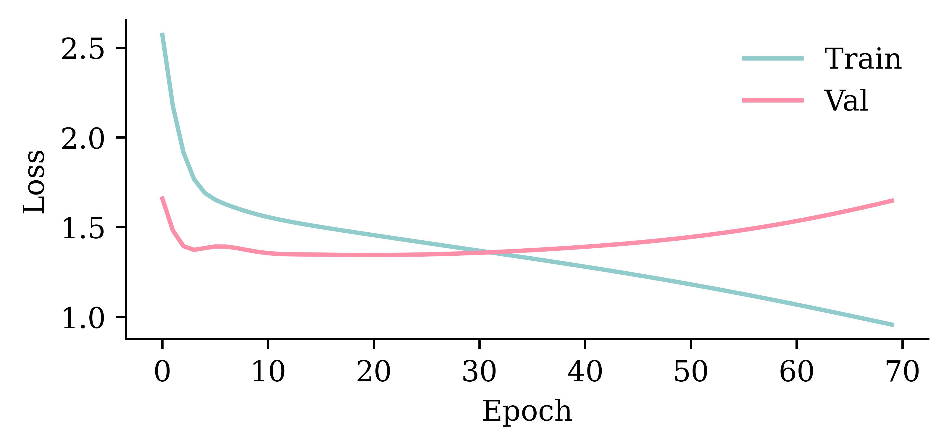

Assess the fits

model_gru.evaluate(val_ds, verbose=0)

1.3462404012680054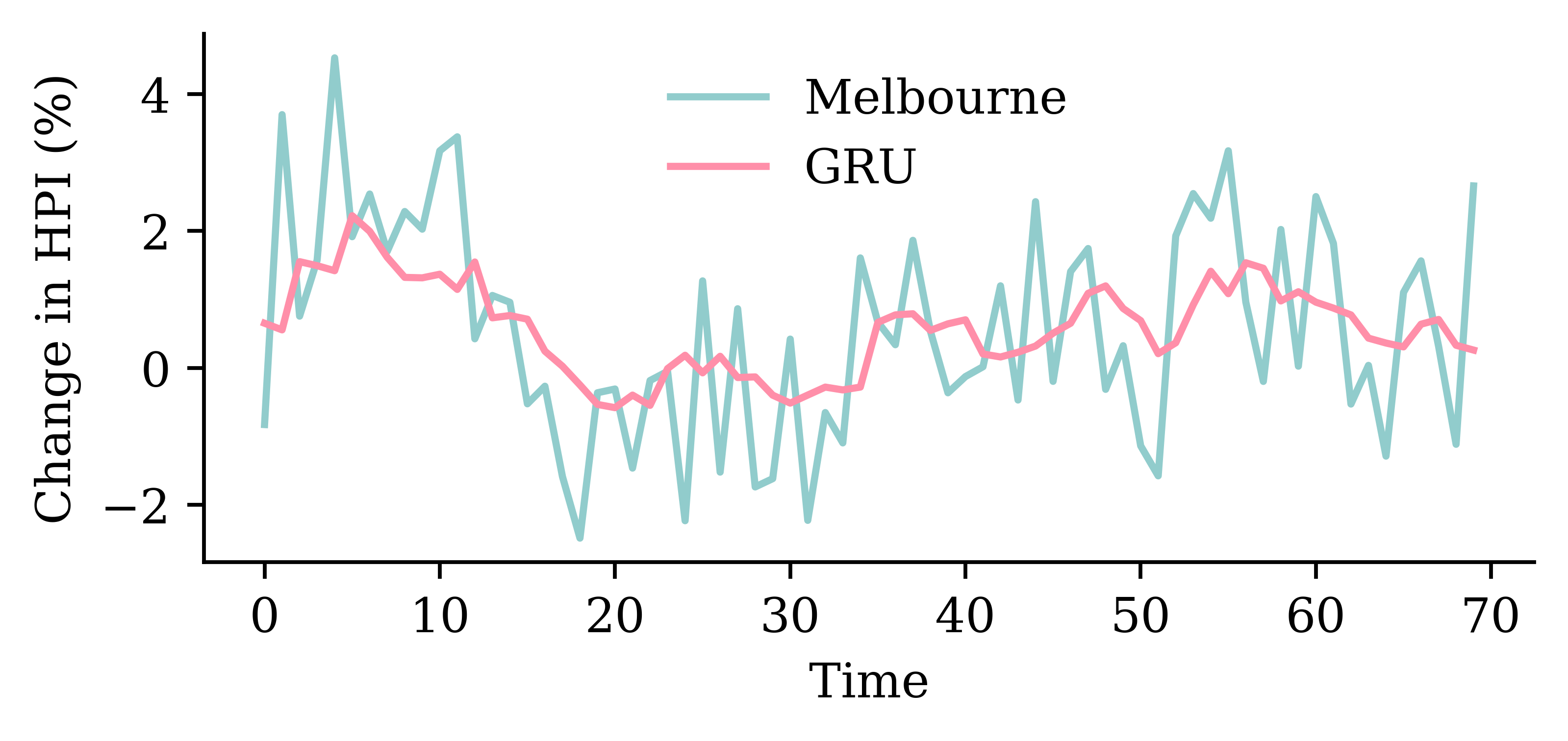

Plotting the predictions

Two `GRU` layers

random.seed(1)

model_two_grus = Sequential([
    Input((seq_length, num_ts)),
    GRU(50, return_sequences=True),
    GRU(50),
    Dense(num_ts, activation="linear")
])

model_two_grus.compile(loss="mse", optimizer="adam")

es = EarlyStopping(patience=50, restore_best_weights=True, verbose=1)

%time hist = model_two_grus.fit(train_ds, epochs=1_000, \
  validation_data=val_ds, callbacks=[es], verbose=0)

Epoch 93: early stopping
Restoring model weights from the end of the best epoch: 43.
CPU times: user 6.14 s, sys: 2.56 s, total: 8.71 s
Wall time: 3.93 s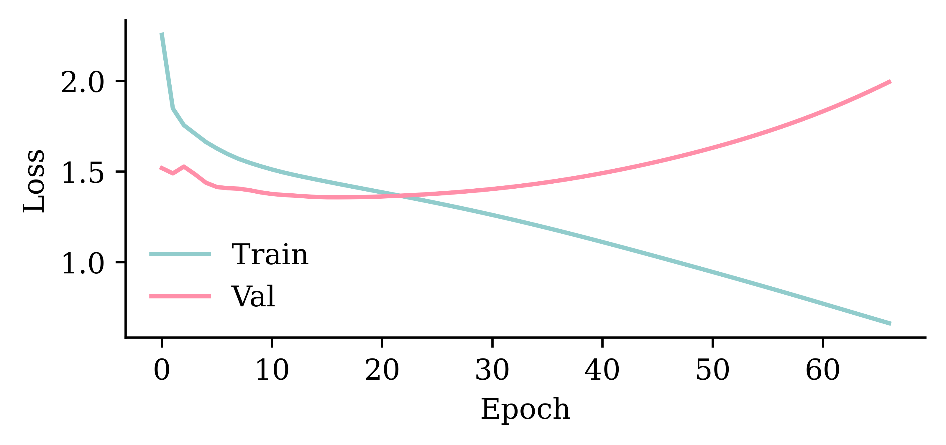

Assess the fits

model_two_grus.evaluate(val_ds, verbose=0)

1.3611823320388794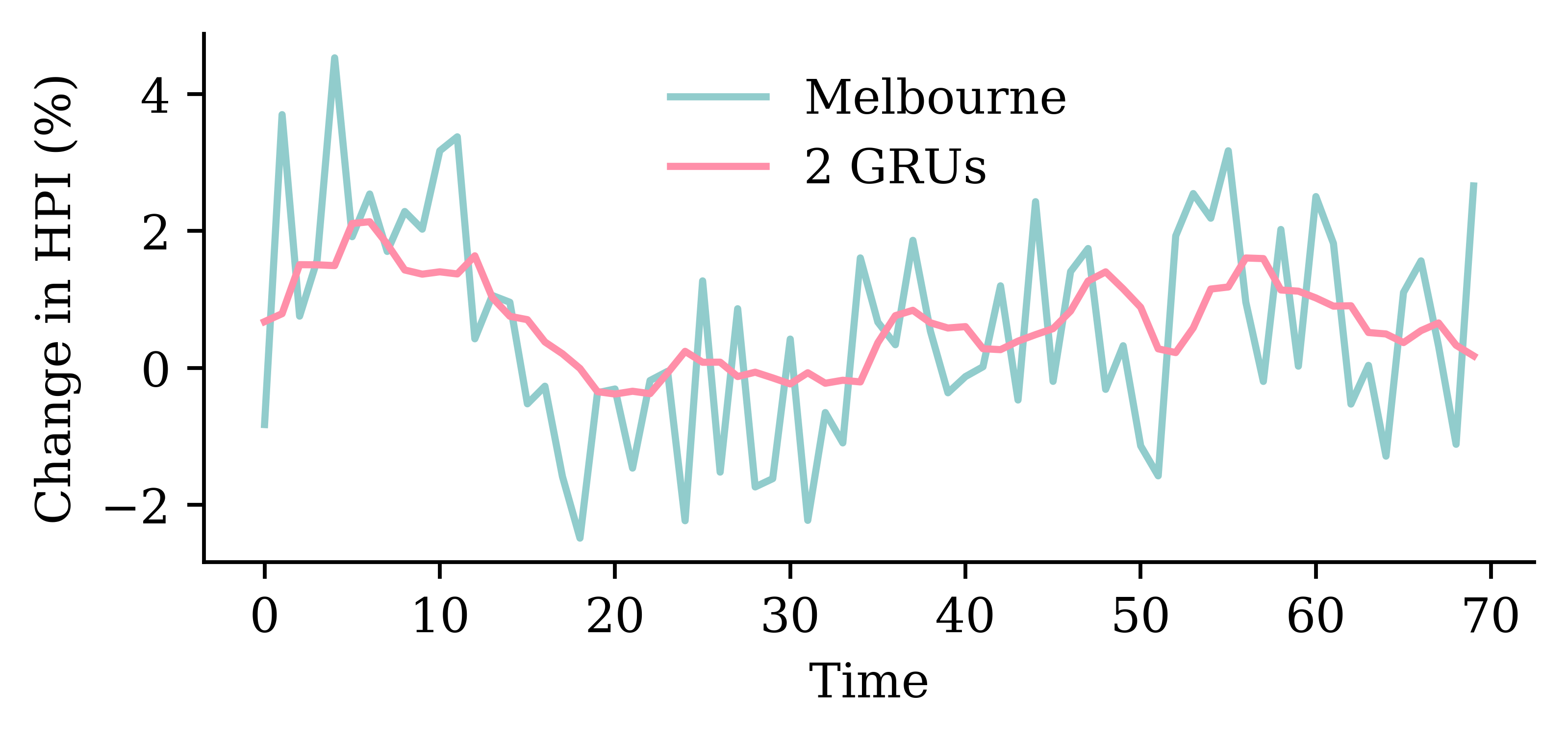

Plotting the predictions

Compare the models

	Model	MSE
1	SimpleRNN	1.628759
0	Dense	1.445832
4	2 GRUs	1.361182
3	GRU	1.346240
2	LSTM	1.343993

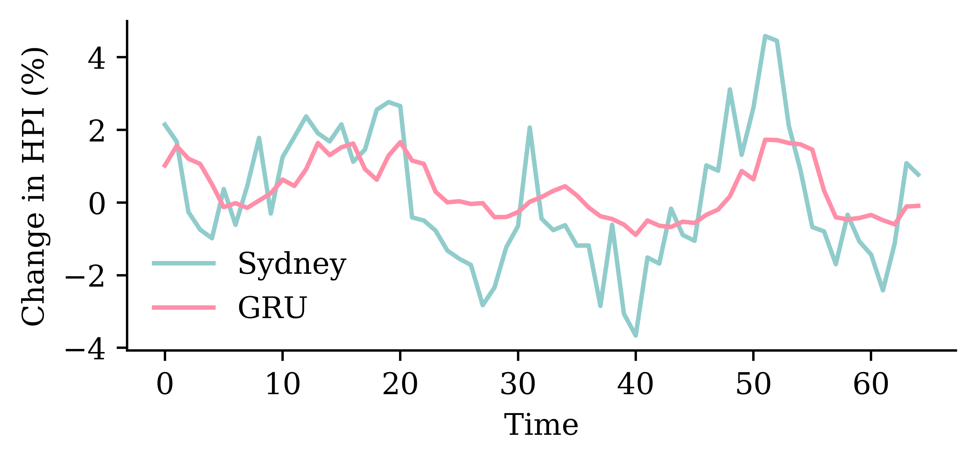
The network with an LSTM layer is the best.

model_lstm.evaluate(test_ds, verbose=0)

1.879453420639038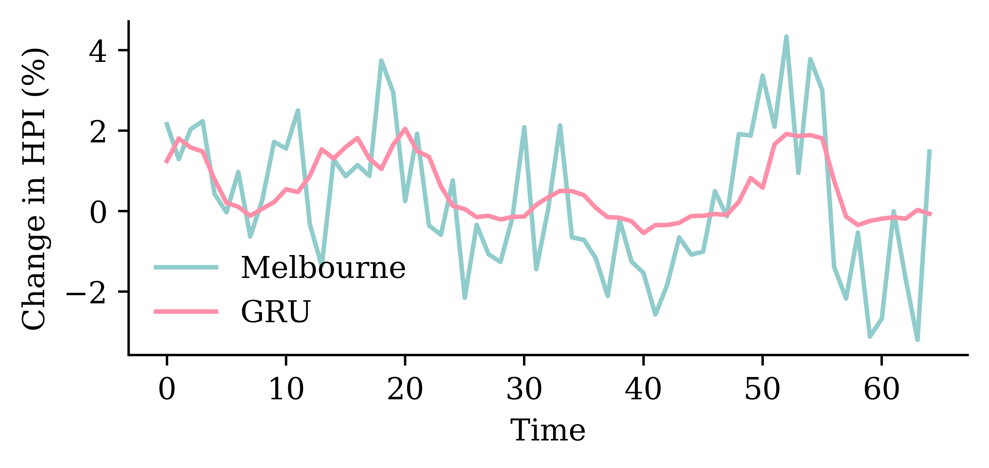

Test set

Package Versions

from watermark import watermark
print(watermark(python=True, packages="keras,matplotlib,numpy,pandas,seaborn,scipy,torch,tensorflow,tf_keras"))

Python implementation: CPython
Python version       : 3.11.8
IPython version      : 8.23.0

keras     : 3.2.0
matplotlib: 3.8.4
numpy     : 1.26.4
pandas    : 2.2.1
seaborn   : 0.13.2
scipy     : 1.11.0
torch     : 2.2.2
tensorflow: 2.16.1
tf_keras  : 2.16.0

Glossary

GRU
LSTM
recurrent neural networks
SimpleRNN

Tensors & Time Series

Shapes of data

The axis argument in numpy

Using axis & keepdims

The rank of a time series

Multivariate time series

Some Recurrent Structures

Recurrence relation

Diagram of an RNN cell

A SimpleRNN cell.

SimpleRNN

SimpleRNN (in batches)

Simple Keras demo

Keras’ SimpleRNN

SimpleRNN weights

LSTM internals

GRU internals

Recurrent Neural Networks

Basic facts of RNNs

Applications

Input and output sequences

Input and output sequences

Input and output sequences

Recurrent layers can be stacked.

CoreLogic Hedonic Home Value Index

Australian House Price Indices

Percentage changes

Percentage changes

The size of the changes

Splitting time series data

Split without shuffling

Subsequences of a time series

On time series splits

On time series splits II

Predicting Sydney House Prices

Creating dataset objects

Converting Dataset to numpy

A dense network

Plot the model

Assess the fits

Plotting the predictions

A SimpleRNN layer

Assess the fits

Plot the model

Plotting the predictions

A LSTM layer

Assess the fits

Plotting the predictions

A GRU layer

Assess the fits

Plotting the predictions

Two GRU layers

Assess the fits

Plotting the predictions

Compare the models

Test set

Predicting Multiple Time Series

Creating dataset objects

Converting Dataset to numpy

A dense network

Plot the model

Assess the fits

Plotting the predictions

A SimpleRNN layer

Assess the fits

Plot the model

Plotting the predictions

A LSTM layer

Assess the fits

Plotting the predictions

A GRU layer

Assess the fits

Plotting the predictions

Two GRU layers

Assess the fits

Plotting the predictions

Compare the models

Test set

Package Versions

Glossary

The `axis` argument in numpy

Using `axis` & `keepdims`

Converting `Dataset` to numpy

A `SimpleRNN` layer

A `LSTM` layer

A `GRU` layer

Two `GRU` layers

Converting `Dataset` to numpy

A `SimpleRNN` layer

A `LSTM` layer

A `GRU` layer

Two `GRU` layers