Generative Networks

ACTL3143 & ACTL5111 Deep Learning for Actuaries

Author

Patrick Laub

Show the package imports

import random
from pathlib import Path

import matplotlib.pyplot as plt
import numpy as np
import numpy.random as rnd
import pandas as pd
import keras
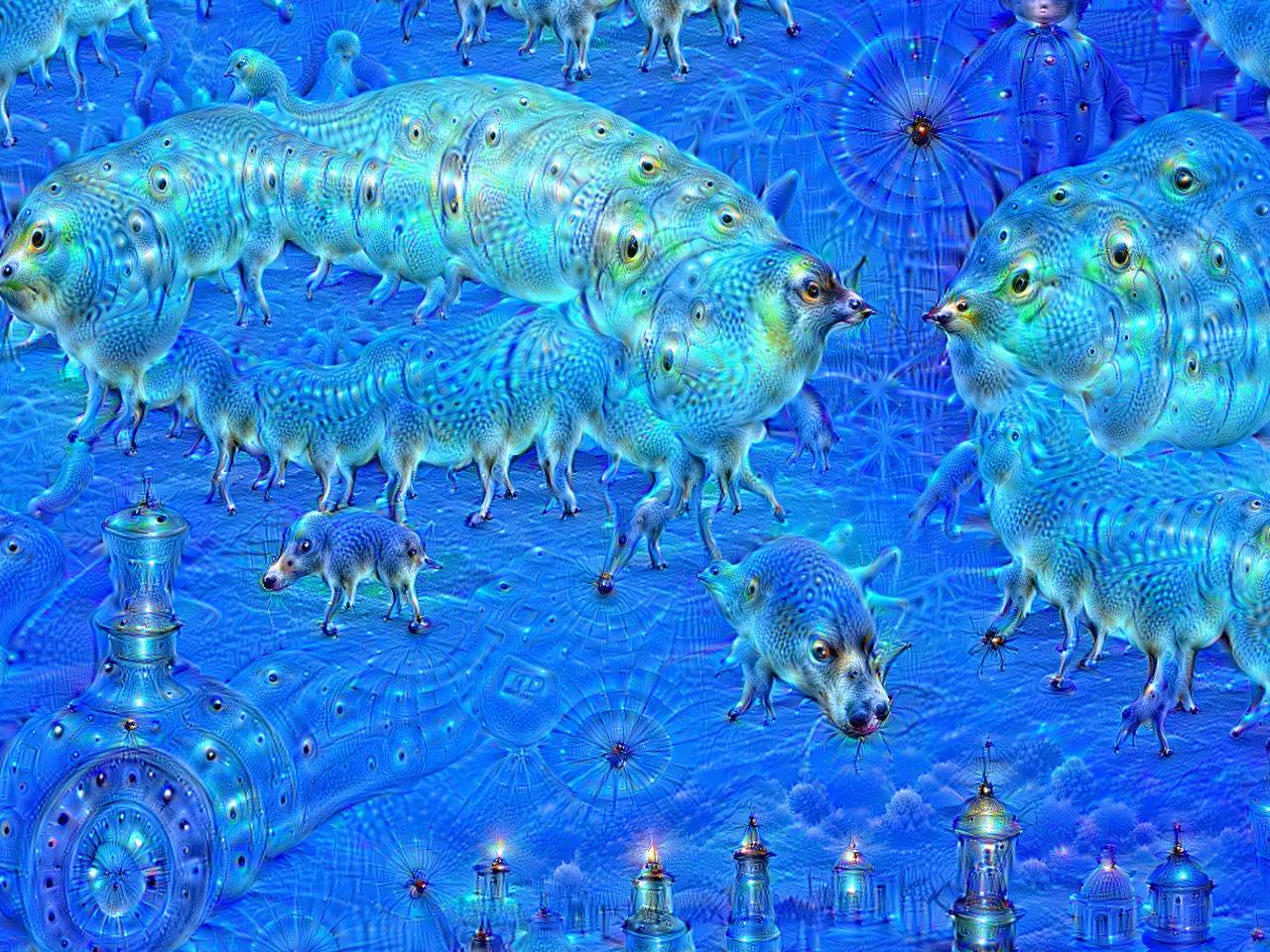
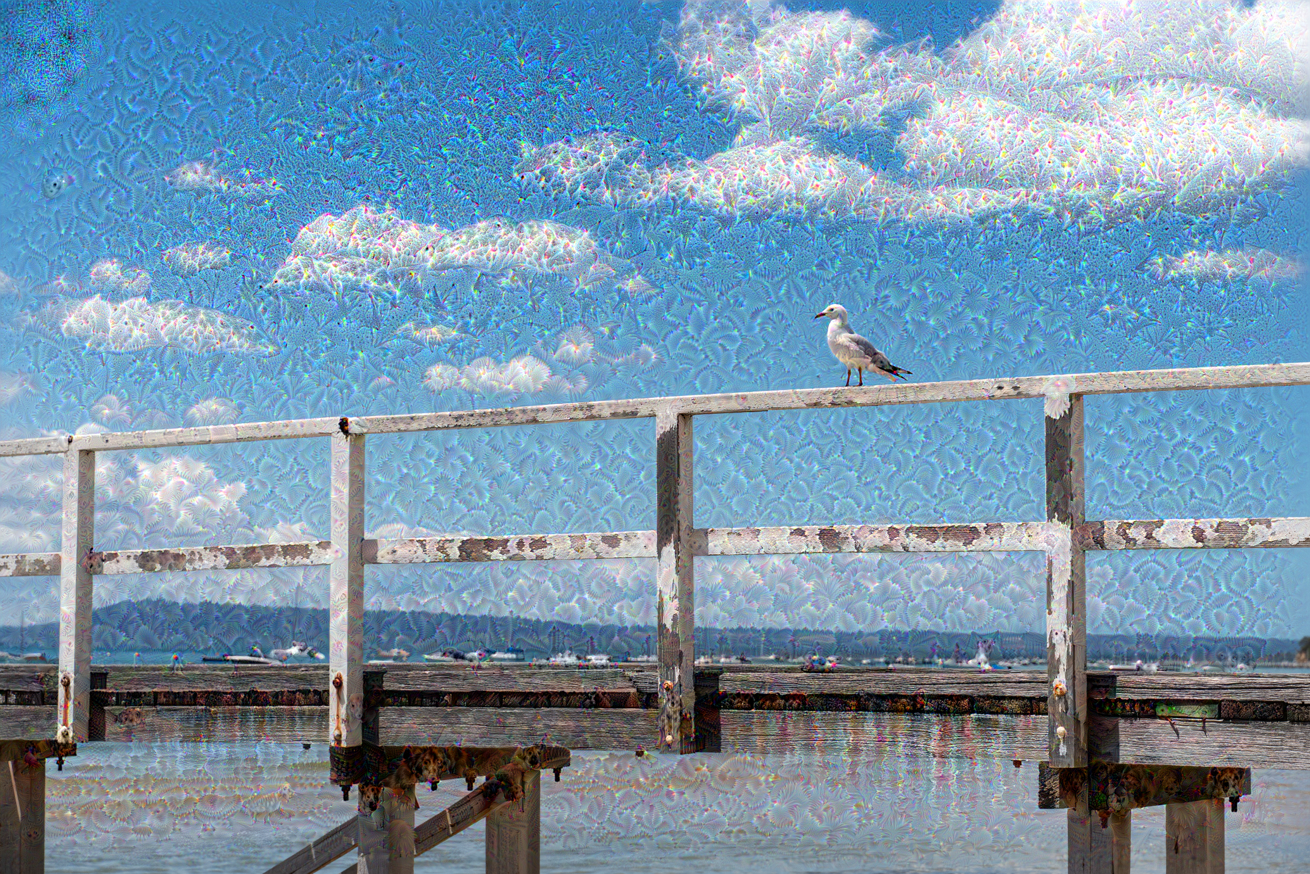
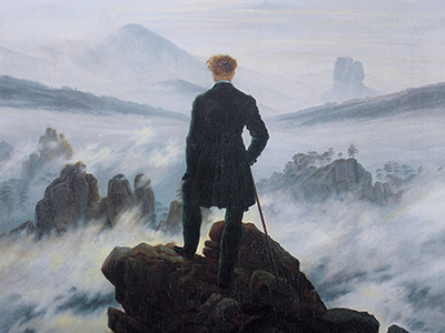
from keras import layers

Text Generation

Generative deep learning

Using AI as augmented intelligence rather than artificial intelligence.
Use of deep learning to augment creative activities such as writing, music and art, to generate new things.
Some applications: text generation, deep dreaming, neural style transfer, variational autoencoders and generative adversarial networks.

Text generation

Generating sequential data is the closest computers get to dreaming.

Generate sequence data: Train a model to predict the next token or next few tokens in a sentence, using previous tokens as input.
A network that models the probability of the next tokens given the previous ones is called a language model.

GPT-3 is a 175 billion parameter text-generation model trained by the startup OpenAI on a large text corpus of digitally available books, Wikipedia and web crawling. GPT-3 made headlines in 2020 due to its capability to generate plausible-sounding text paragraphs on virtually any topic.

Word-level language model

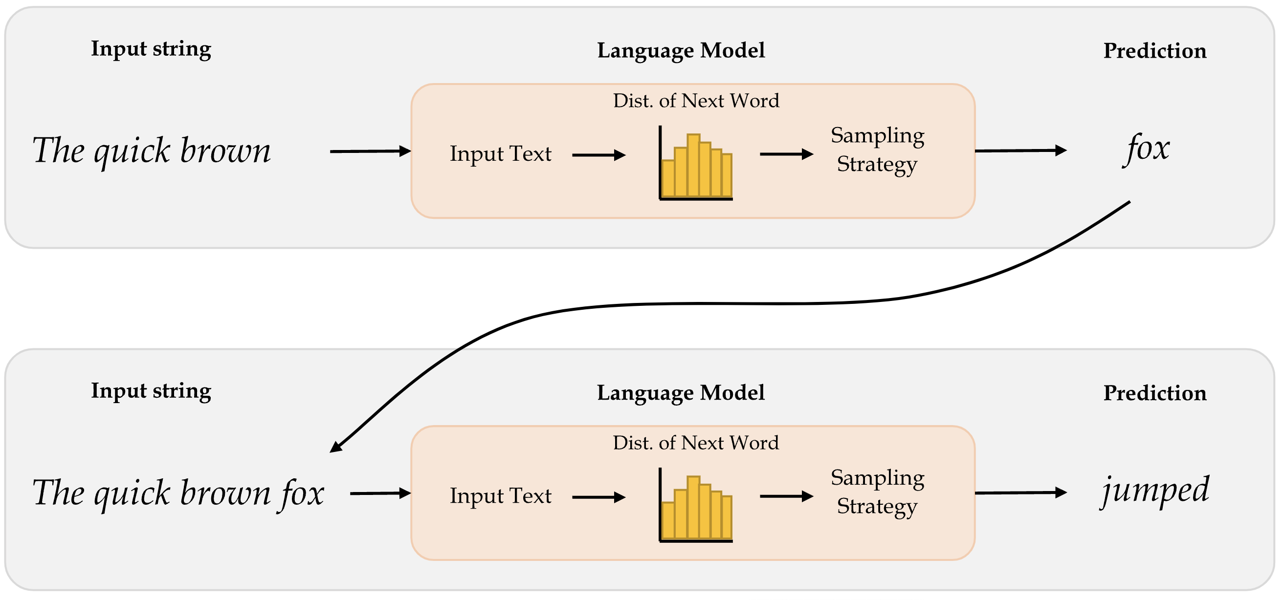
The way how word-level language models work is that, it first takes in the input text and then generates the probability distribution of the next word. This distribution tells us how likely a certain word is to be the next word. Thereafter, the model implements a appropriate sampling strategy to select the next word. Once the next word is predicted, it is appended to the input text and then passed in to the model again to predict the next word. The idea here is to predict the word after word.

Character-level language model

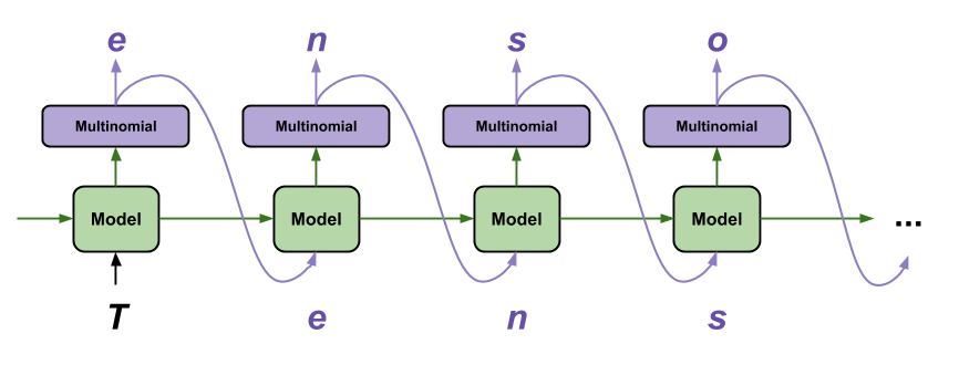
Character-level language predtics the next character given a certain input character. They capture patterns at a much granular level and do not aim to capture semantics of words.

Useful for speech recognition

RNN output	Decoded Transcription
what is the weather like in bostin right now	what is the weather like in boston right now
prime miniter nerenr modi	prime minister narendra modi
arther n tickets for the game	are there any tickets for the game

Figure 1: Examples of transcriptions directly from the RNN with errors that are fixed by addition of a language model.

The above example shows how RNN predictions (for sequential data processing) can be improved by fixing errors using a language model.

Generating Shakespeare I

The following is an example how a language model trained on works of Shakespeare starts predicting words after we input a string. This is an example of a character-level prediction, where we aim to predict the most likely character, not the word.

ROMEO:
Why, sir, what think you, sir?

AUTOLYCUS:
A dozen; shall I be deceased.
The enemy is parting with your general,
As bias should still combit them offend
That Montague is as devotions that did satisfied;
But not they are put your pleasure.

Generating Shakespeare II

DUKE OF YORK:
Peace, sing! do you must be all the law;
And overmuting Mercutio slain;
And stand betide that blows which wretched shame;
Which, I, that have been complaints me older hours.

LUCENTIO:
What, marry, may shame, the forish priest-lay estimest you, sir,
Whom I will purchase with green limits o’ the commons’ ears!

Generating Shakespeare III

ANTIGONUS:
To be by oath enjoin’d to this. Farewell!
The day frowns more and more: thou’rt like to have
A lullaby too rough: I never saw
The heavens so dim by day. A savage clamour!

[Exit, pursued by a bear]

Sampling strategy

The sampling strategy refers to the way how we pick the next word/character as the prediction after observing the distribution. There are different sampling strategies and they aim to serve different levels of trade-offs between exploration and exploitation when generating text sequences.

Greedy sampling will choose the token with the highest probability. It makes the resulting sentence repetitive and predictable.
Stochastic sampling: if a word has probability 0.3 of being next in the sentence according to the model, we’ll choose it 30% of the time. But the result is still not interesting enough and still quite predictable.
Use a softmax temperature to control the randomness. More randomness results in more surprising and creative sentences.

Softmax temperature

The softmax temperature is a parameter that controls the randomness of the next token.
The formula is: \text{softmax}_\text{temperature}(x) = \frac{\exp(x / \text{temperature})}{\sum_i \exp(x_i / \text{temperature})}

“I am a” …

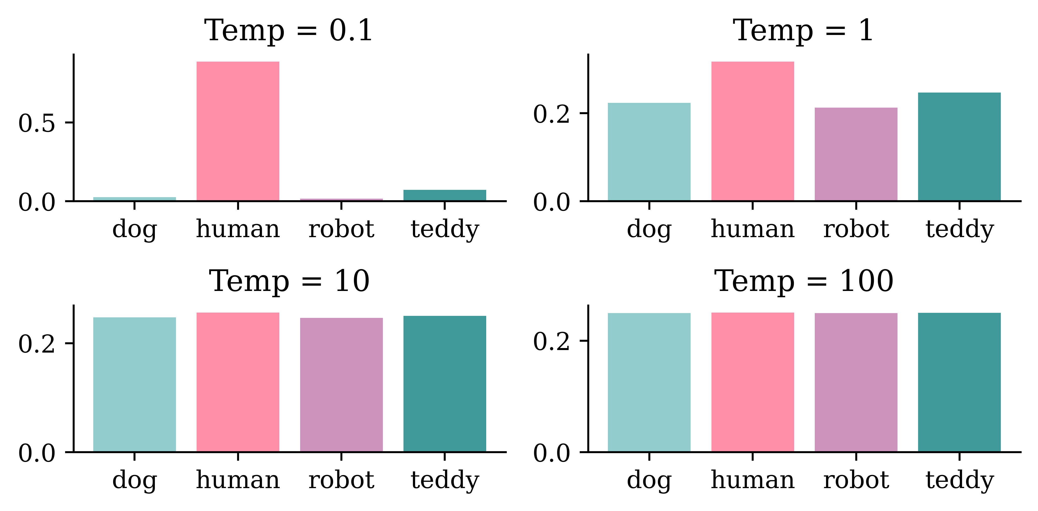
The graphical illustration above shows how the distribution of words change with different levels of Temp values. Higher levels of temperatures result in less predictable(more interesting) outcomes. If we continue to increase the Temp levels, after a certain point, outcomes will be picked completely at random. This predictions after this point might not be meaningful. Hence, attention to the trade-off between predictability and interestingness is important when deciding the Temp levels.

The following sections show how a neural network turned on the same dataset, and given the same starting input string In today’s lecture we will shall generate very different sequences of text as predictions. Temp=0.25 may give interesting outputs compared to Temp=0.01 and Temp=0.50 may give interesting outputs compared to Temp=0.25. However, when we keep on increasing Temp levels, the neural network starts giving out random(meaningless) outcomes.

Generating Laub (temp = 0.01)

In today’s lecture we will be different situation. So, next one is what they rective that each commit to be able to learn some relationships from the course, and that is part of the image that it’s very clese and black problems that you’re trying to fit the neural network to do there instead of like a specific though shef series of layers mean about full of the chosen the baseline of car was in the right, but that’s an important facts and it’s a very small summary with very scrort by the beginning of the sentence.

Generating Laub (temp = 0.25)

In today’s lecture we will decreas before model that we that we have to think about it, this mightsks better, for chattely the same project, because you might use the test set because it’s to be picked up the things that I wanted to heard of things that I like that even real you and you’re using the same thing again now because we need to understand what it’s doing the same thing but instead of putting it in particular week, and we can say that’s a thing I mainly link it’s three columns.

Generating Laub (temp = 0.5)

In today’s lecture we will probably the adw n wait lots of ngobs teulagedation to calculate the gradient and then I’ll be less than one layer the next slide will br input over and over the threshow you ampaigey the one that we want to apply them quickly. So, here this is the screen here the main top kecw onct three thing to told them, and the output is a vertical variables and Marceparase of things that you’re moving the blurring and that just data set is to maybe kind of categorical variants here but there’s more efficiently not basically replace that with respect to the best and be the same thing.

Generating Laub (temp = 1)

In today’s lecture we will put it different shates to touch on last week, so I want to ask what are you object frod current. They don’t have any zero into it, things like that which mistakes. 10 claims that the average version was relden distever ditgs and Python for the whole term wo long right to really. The name of these two options. There are in that seems to be modified version. If you look at when you’re putting numbers into your, that that’s over. And I went backwards, up, if they’rina functional pricing working with.

Generating Laub (temp = 1.5)

In today’s lecture we will put it could be bedinnth. Lowerstoriage nruron. So rochain the everything that I just sGiming. If there was a large. It’s gonua draltionation. Tow many, up, would that black and 53% that’s girter thankAty will get you jast typically stickK thing. But maybe. Anyway, I’m going to work on this libry two, past, at shit citcs jast pleming to memorize overcamples like pre pysing, why wareed to smart a one in this reportbryeccuriay.

Generate the most likely sequence

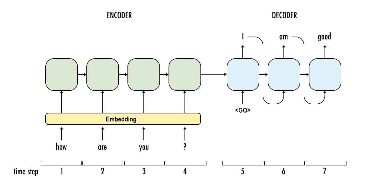
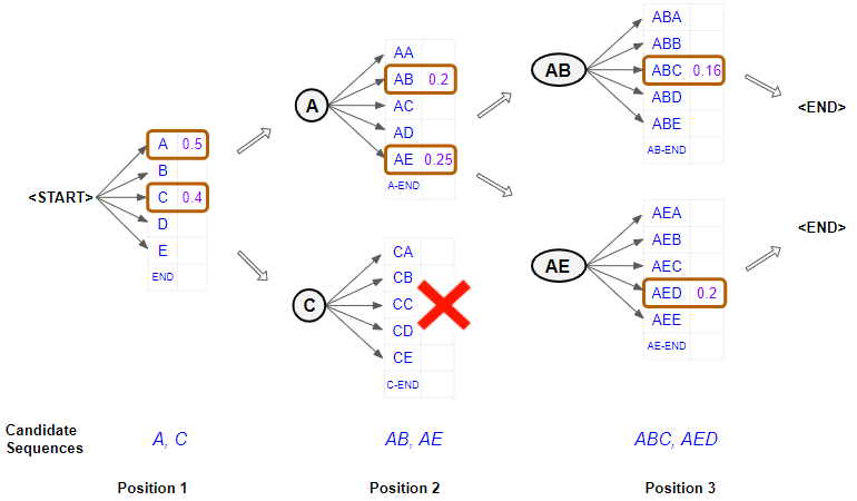
Similar to other sequence generating tasks such as generating the next word or generating the next character, generating an entire sequence of words is also useful. The task involves generating the most likely sequence after observing model predictions.

An example sequence-to-sequence chatbot model.

Beam search

Instead of trying to carry forward only the highest probable prediction, beam search carries forward several high probable predictions, and then decide the highest probable combination of predictions. Beam search helps expand the exploration horizon for predictions which can contribute to more contextually relevant model predictions. However, this comes at a certain computational complexity.

Transformers

Transformers are a special type of neural networks that are proven to be highly effective in NLP tasks. They can capture long-run dependencies in the sequential data that is useful for generating predictions with contextual meaning. It makes use of the self-attention mechanism which studies all inputs in the sequence together, tries to understand the dependencies among them, and then utilizes the information about long-run dependencies to predict the output sequence.

Transformer architecture

GPT makes use of a mechanism known as attention, which removes the need for recurrent layers (e.g., LSTMs). It works like an information retrieval system, utilizing queries, keys, and values to decide how much information it wants to extract from each input token.

Attention heads can be grouped together to form what is known as a multihead attention layer. These are then wrapped up inside a Transformer block, which includes layer normalization and skip connections around the attention layer. Transformer blocks can be stacked to create very deep neural networks.

Transformer architecture reference

🤗 Transformers package

The following code uses transformers library from Hugging Face to create a text generation pipeline using the GPT2 (Generative Pre-trained Transformer 2).

1import transformers
2from transformers import pipeline
3generator = pipeline(task="text-generation", model="gpt2", revision="6c0e608")

1: Imports the transformers library
2: Imports the class pipeline
3: Creates a pipeline object called the generator, whose task would be to generate text, using the pretrained model GPT2. revision="6c0e608" specifies the specific revision of the model to refer

1transformers.set_seed(1)
2print(generator("It's the holidays so I'm going to enjoy")[0]["generated_text"])

1: Sets the seed for reproducibility
2: Applies the generator object to generate a text based on the input It’s the holidays so I’m going to enjoy. The result from genrator would be a list of generated texts. To select the first output sequence hence, we pass the command [0]["generated_text"]

Setting `pad_token_id` to `eos_token_id`:50256 for open-end generation.

It's the holidays so I'm going to enjoy the rest of the time and look forward to this week with new friends!"

We can try the same code with a different seed value, and it would give a very different output.

transformers.set_seed(2)
print(generator("It's the holidays so I'm going to enjoy")[0]["generated_text"])

Setting `pad_token_id` to `eos_token_id`:50256 for open-end generation.

It's the holidays so I'm going to enjoy them again."

I'm not making any assumptions.

I am very happy. It's the holidays so I'm going to enjoy them again. — Daniel Nasser (@DanielN

Reading the course profile

Another application of pipeline is the ability to generate texts in the answer format. The following is an example of how a pretrained model can be used to answer questions by relating it to a body of text information(context).

context = """
StoryWall Formative Discussions: An initial StoryWall, worth 2%, is due by noon on June 3. The following StoryWalls are worth 4% each (taking the best 7 of 9) and are due at noon on the following dates:
The project will be submitted in stages: draft due at noon on July 1 (10%), recorded presentation due at noon on July 22 (15%), final report due at noon on August 1 (15%).

As a student at UNSW you are expected to display academic integrity in your work and interactions. Where a student breaches the UNSW Student Code with respect to academic integrity, the University may take disciplinary action under the Student Misconduct Procedure. To assure academic integrity, you may be required to demonstrate reasoning, research and the process of constructing work submitted for assessment.
To assist you in understanding what academic integrity means, and how to ensure that you do comply with the UNSW Student Code, it is strongly recommended that you complete the Working with Academic Integrity module before submitting your first assessment task. It is a free, online self-paced Moodle module that should take about one hour to complete.

StoryWall (30%)

The StoryWall format will be used for small weekly questions. Each week of questions will be released on a Monday, and most of them will be due the following Monday at midday (see assessment table for exact dates). Students will upload their responses to the question sets, and give comments on another student's submission. Each week will be worth 4%, and the grading is pass/fail, with the best 7 of 9 being counted. The first week's basic 'introduction' StoryWall post is counted separately and is worth 2%.

Project (40%)

Over the term, students will complete an individual project. There will be a selection of deep learning topics to choose from (this will be outlined during Week 1).

The deliverables for the project will include: a draft/progress report mid-way through the term, a presentation (recorded), a final report including a written summary of the project and the relevant Python code (Jupyter notebook).

Exam (30%)

The exam will test the concepts presented in the lectures. For example, students will be expected to: provide definitions for various deep learning terminology, suggest neural network designs to solve risk and actuarial problems, give advice to mock deep learning engineers whose projects have hit common roadblocks, find/explain common bugs in deep learning Python code.
"""

Question answering

1qa = pipeline("question-answering", model="distilbert-base-cased-distilled-squad", revision="626af31")

1: Creates a question and answer style pipeline object by referring to the pretrained model pre-trained DistilBERT model (fine-tuned on the SQuAD: Stanford Question Answering Dataset) with revision 626af31

1qa(question="What weight is the exam?", context=context)

1: Answers the questions What weight is the exam given the context specified

{'score': 0.501968264579773, 'start': 2092, 'end': 2095, 'answer': '30%'}

qa(question="What topics are in the exam?", context=context)

{'score': 0.2127578854560852,
 'start': 1778,
 'end': 1791,
 'answer': 'deep learning'}

qa(question="When is the presentation due?", context=context)

{'score': 0.5296494364738464,
 'start': 1319,
 'end': 1335,
 'answer': 'Monday at midday'}

qa(question="How many StoryWall tasks are there?", context=context)

{'score': 0.21390870213508606, 'start': 1155, 'end': 1158, 'answer': '30%'}

ChatGPT is Transformer + RLHF

At the time of writing, there is no official paper that describes how ChatGPT works in detail, but from the official blog post we know that it uses a technique called reinforcement learning from human feedback (RLHF) to fine-tune the GPT-3.5 model.

ChatGPT internals

ChatGPT

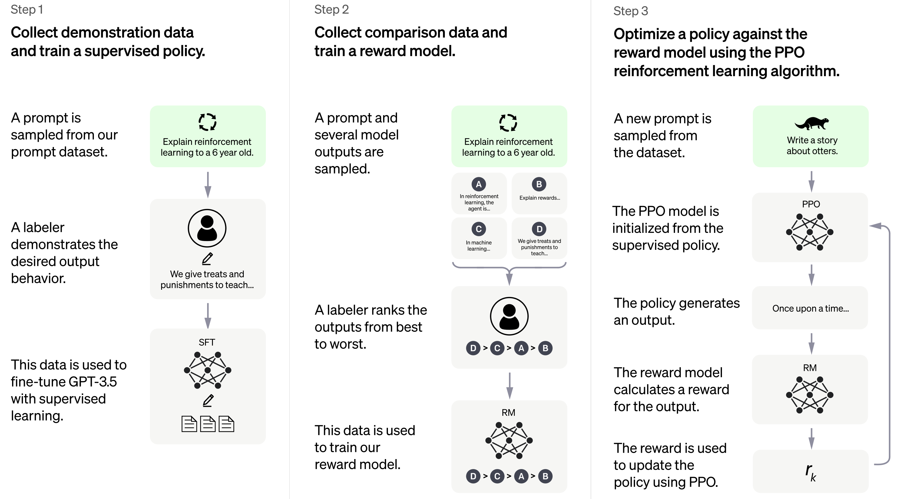
While ChatGPT still has many limitations (such as sometimes “hallucinating” factually incorrect information), it is a powerful example of how Transformers can be used to build generative models that can produce complex, long-ranging, and novel output that is often indistinguishable from human-generated text. The progress made thus far by models like ChatGPT serves as a testament to the potential of AI and its transformative impact on the world.

Image Generation

Reverse-engineering a CNN

Reverse engineering is a process where we manipulate the inputs x while keeping the loss function and the model architecture the same. This is useful in understanding the inner workings of the model, especially when we do not have access to the model architecture or the original train dataset. The idea here is to tweak/distort the input feature data and observe how model predictions vary. This provides meaningful insights in to what patterns in the input data are most critical to making model predictions.

This task however requires computing the gradients of the model’s outputs with respect to all input features, hence, can be time consuming.

A CNN is a function f_{\boldsymbol{\theta}}(\mathbf{x}) that takes a vector (image) \mathbf{x} and returns a vector (distribution) \widehat{\mathbf{y}}.

Normally, we train it by modifying \boldsymbol{\theta} so that

\boldsymbol{\theta}^*\ =\ \underset{\boldsymbol{\theta}}{\mathrm{argmin}} \,\, \text{Loss} \bigl( f_{\boldsymbol{\theta}}(\mathbf{x}), \mathbf{y} \bigr).

However, it is possible to not train the network but to modify \mathbf{x}, like

\mathbf{x}^*\ =\ \underset{\mathbf{x}}{\mathrm{argmin}} \,\, \text{Loss} \bigl( f_{\boldsymbol{\theta}}(\mathbf{x}), \mathbf{y} \bigr).

This is very slow as we do gradient descent every single time.

Adversarial examples

An adversarial attack refers to a small carefully created modifications to the input data that aims to trick the model in to making wrong predictions while keeping the y_true same. The goal is to identify instances where subtle modifications in the input data (which are not instantaneously recognized) can lead to erroneous model predictions.

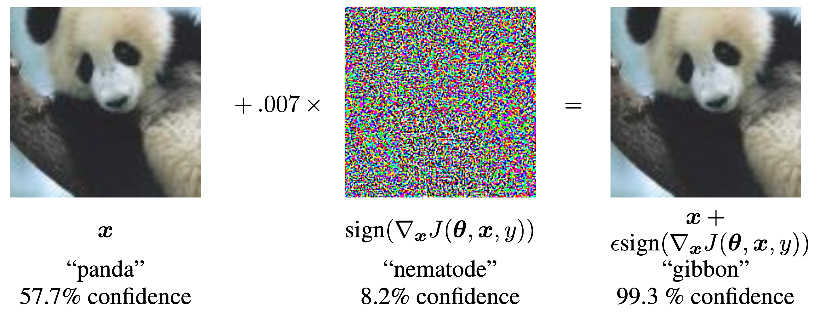
A demonstration of fast adversarial example generation applied to GoogLeNet on ImageNet. By adding an imperceptibly small vector whose elements are equal to the sign of the elements of the gradient of the cost function with respect to the input, we can change GoogLeNet’s classification of the image.

The above example shows how a small perturbation to the image of a panda led to the model predicting the image as a gibbon with high confidence. This indicates that there may be certain patterns in the data which are not clearly seen by the human eye, but the model is relying on them to make predictions. Identifying these sensitivities/vulnerabilities are important to understand how a model is making its predictions.

Adversarial stickers

The above graphical illustration shows how adding a metal component changes the model predictions from Banana to toaster with high confidence.

Adversarial text

Adversarial attacks on text generation models help users get an understanding of the inner workings NLP models. This includes identifying input patterns that are critical to model predictions, and assessing performance of NLP models for robustness.

“TextAttack 🐙 is a Python framework for adversarial attacks, data augmentation, and model training in NLP”

Deep Dream

DeepDream

Even though many deep learning models are black boxes, convnets are quite interpretable via visualization. Some visualization techniques are: visualizing convnet outputs shows how convnet layers transform the input, visualizing convnet filters shows what visual patterns or concept each filter is receptive to, etc.
The activations of the first few layers of the network carries more information about the visual contents, while deeper layers encode higher, more abstract concepts.

DeepDream

Each filter is receptive to a visual pattern. To visualize a convnet filter, gradient ascent is used to maximize the response of the filter. Gradient ascent maximize a loss function and moves the image in a direction that activate the filter more strongly to enhance its reading of the visual pattern.
DeepDream maximizes the activation of the entire convnet layer rather than that of a specific filter, thus mixing together many visual patterns all at once.
DeepDream starts with an existing image, latches on to preexisting visual patterns, distorting elements of the image in a somewhat artistic fashion.

Original

A sunny day on the Mornington peninsula.

Transformed

Neural style transfer

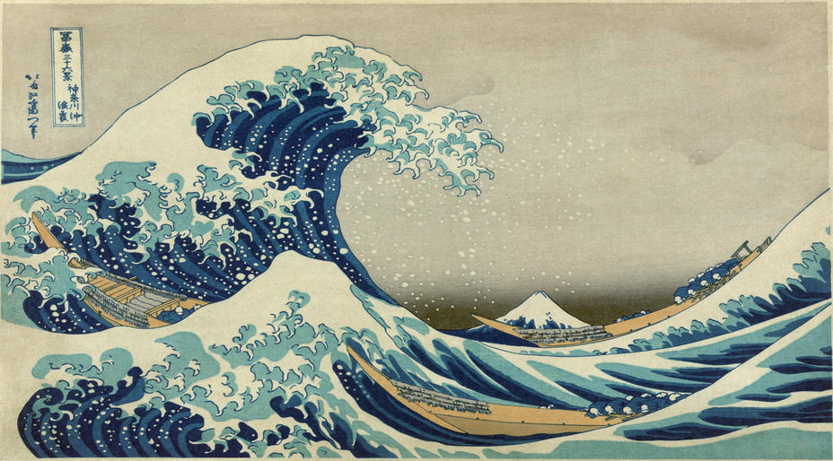
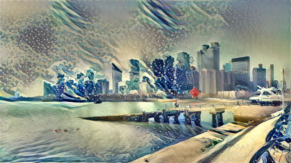
Applying the style of a reference image to a target image while conserving the content of the target image.

Style: textures, colors, visual patterns (blue-and-yellow circular brushstrokes in Vincent Van Gogh’s Starry Night)
Content: the higher-level macrostructure of the image (buildings in the Tübingen photograph).

Goal of NST

What the model does:

Preserve content by maintaining similar deeper layer activations between the original image and the generated image. The convnet should “see” both the original image and the generated image as containing the same things.
Preserve style by maintaining similar correlations within activations for both low level layers and high-level layers. Feature correlations within a layer capture textures: the generated image and the style-reference image should share the same textures at different spatial scales.

A wanderer in Greenland

Content

Style

*Wanderer above the Sea of Fog* by Caspar David Friedrich.

A wanderer in Greenland II

Question

How would you make this faster for one specific style image?

A new style image

A new content image

Another neural style transfer

The seascape in Qingdao in the style of Hokusai’s Great Wave off Kanagawa

Why is this important?

Taking derivatives with respect to the input image can be a first step toward explainable AI for convolutional networks.

Autoencoders

Autoencoder

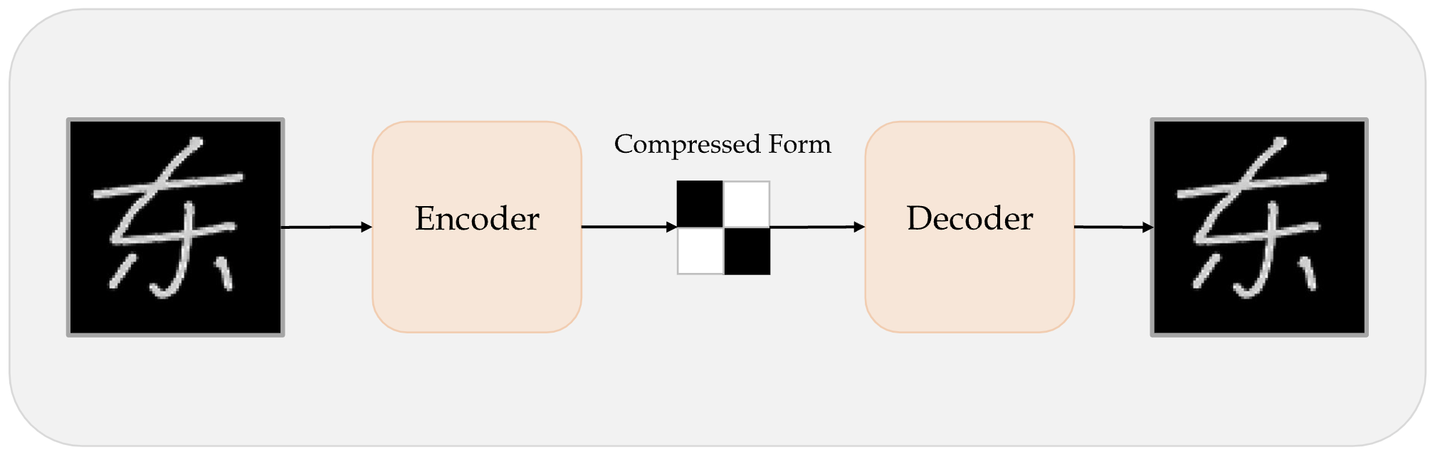
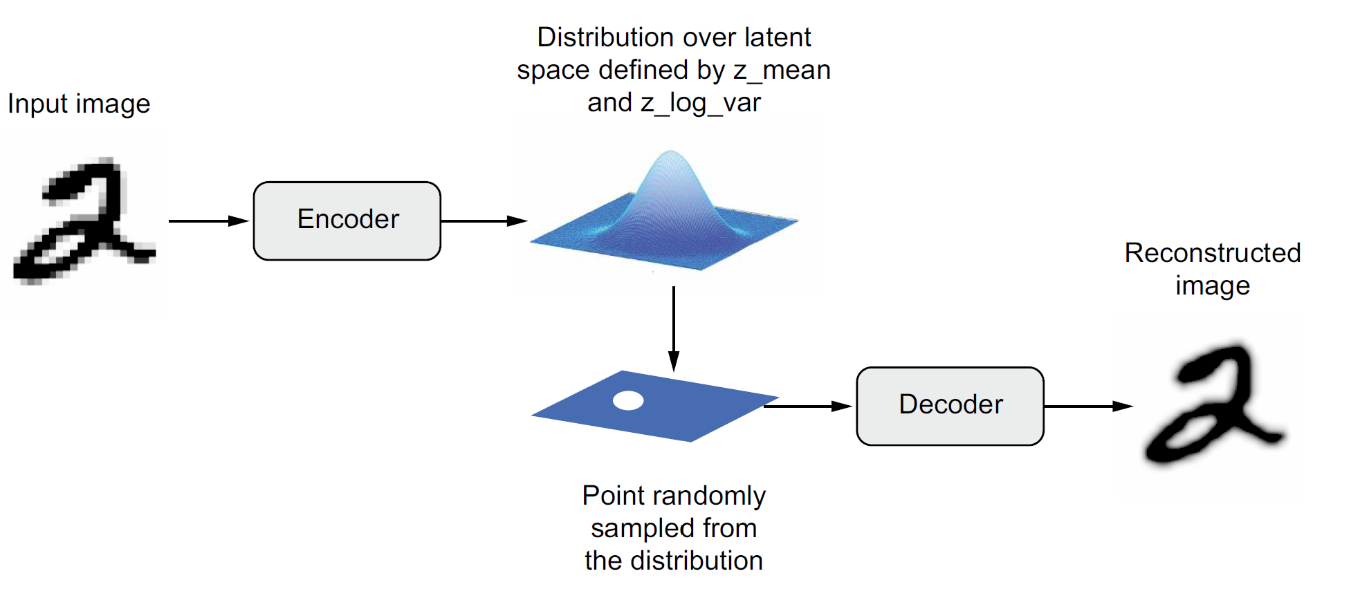
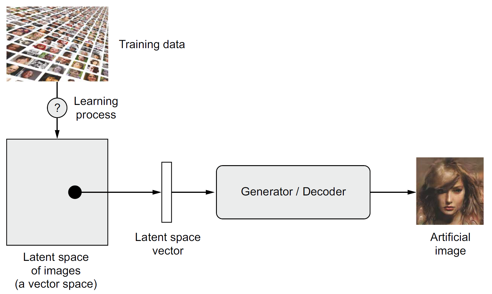
An autoencoder takes a data/image, maps it to a latent space via an encoder module, then decodes it back to an output with the same dimensions via a decoder module.

They are useful in learning latent representations of the data.

Autoencoder II

An autoencoder is trained by using the same image as both the input and the target, meaning an autoencoder learns to reconstruct the original inputs. Therefore it’s not supervised learning, but self-supervised learning.
If we impose constraints on the encoders to be low-dimensional and sparse, the input data will be compressed into fewer bits of information.
Latent space is a place that stores low-dimensional representation of data. It can be used for data compression, where data is compressed to a point in a latent space.
An image can be compressed into a latent representation, which can then be reconstructed back to a slightly different image.

For image editing, an image can be projected onto a latent space and moved inside the latent space in a meaningful way (which means we modify its latent representation), before being mapped back to the image space. This will edit the image and allow us to generate images that have never been seen before.

Example: PSAM

Loading the dataset off-screen (using Lecture 6 code).

plt.imshow(X_train[0], cmap="gray");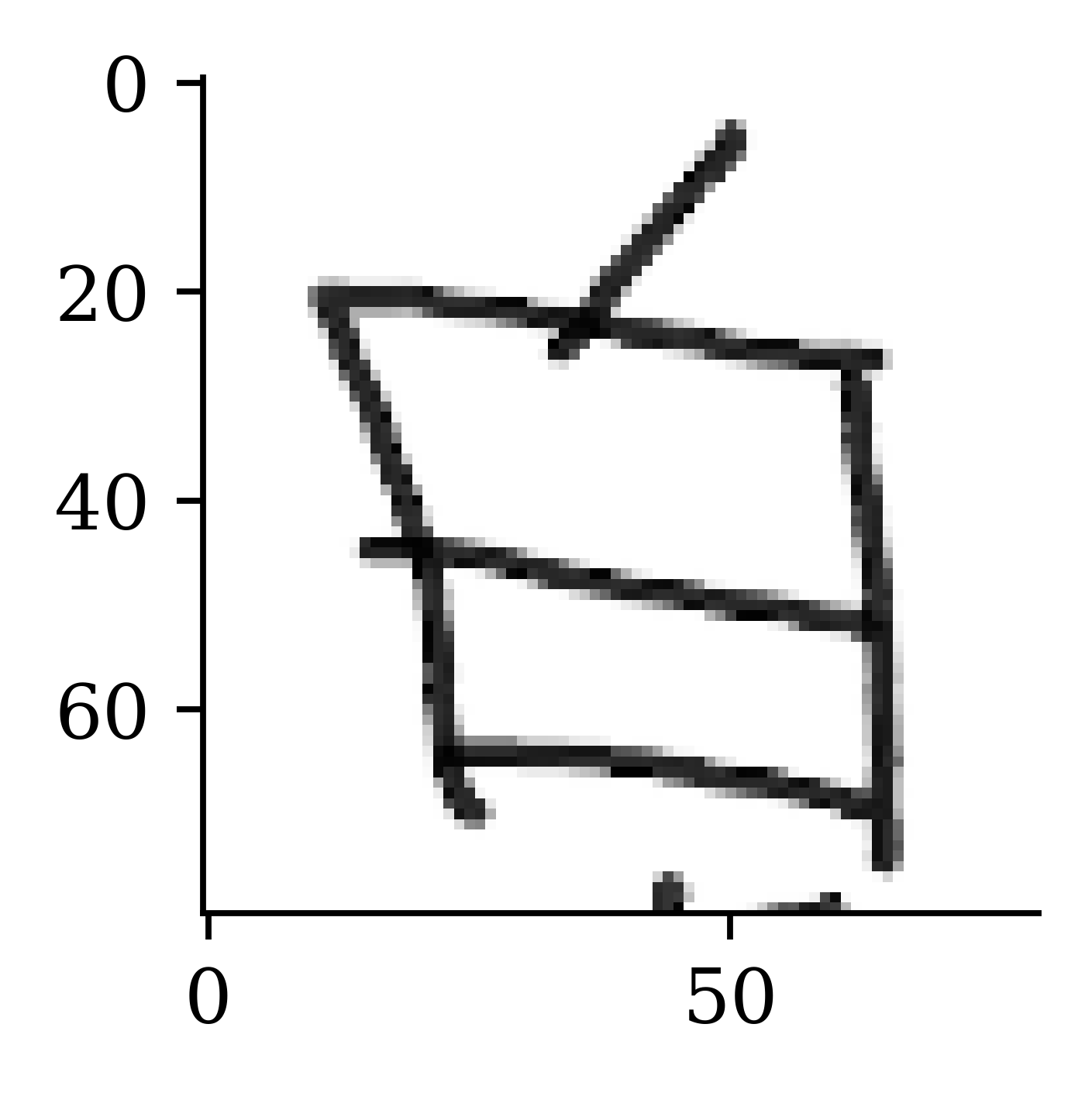

plt.imshow(X_train[42], cmap="gray");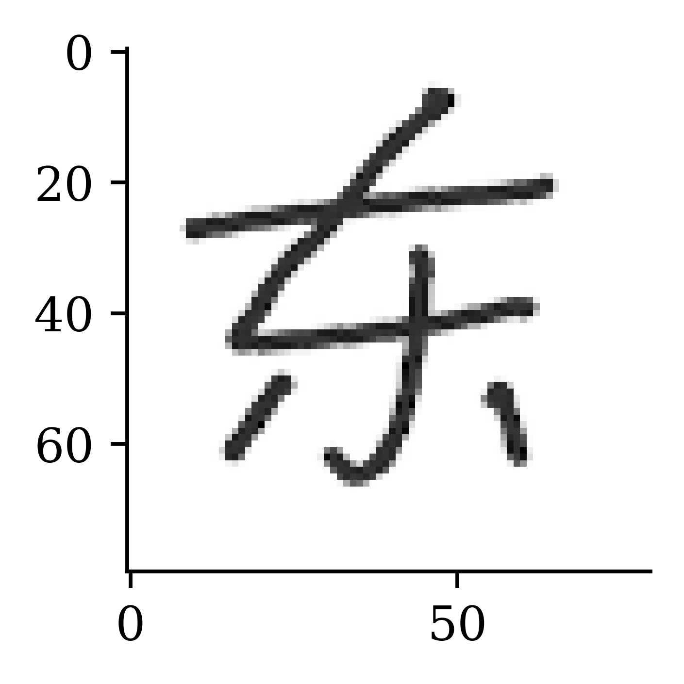

A compression game

Encoding is the overall process of compressing an input with containing data in a high dimensional space to a low dimension space. Compressing is the action of identifying necessary information in the data (versus redundant data) and representing the input in a more concise form. The following slides show two different ways of representing the same data. The second representation is more concise (and smarter) than the first.

plt.imshow(X_train[42], cmap="gray");
print(img_width * img_height)

A 4 with a curly foot, a flat line goes across the middle of the 4, two feet come off the bottom.

96 characters

A Dōng character, rotated counterclockwise 15 degrees.

54 characters

Make a basic autoencoder

The following code is an example of constructing a basic autoencoder. The high-level idea here is to take an image, compress the information of the image from 6400 pixels to 400 pixels (encoding stage) and decode it back to the original image size (decoding stage). Note that we train the neural network keeping the input and the output the same.

num_hidden_layer = 400
print(f"Compress from {img_height * img_width} pixels to {num_hidden_layer} latent variables.")

Compress from 6400 pixels to 400 latent variables.

1random.seed(123)

model = keras.models.Sequential([
    layers.Input((img_height, img_width, 1)),
2    layers.Rescaling(1./255),
3    layers.Flatten(),
4    layers.Dense(num_hidden_layer, "relu"),
5    layers.Dense(img_height*img_width, "sigmoid"),
6    layers.Reshape((img_height, img_width, 1)),
7    layers.Rescaling(255),
])

8model.compile("adam", "mse")
9epochs = 1_000
es = keras.callbacks.EarlyStopping(
10    patience=5, restore_best_weights=True)
model.fit(X_train, X_train, epochs=epochs, verbose=0,
11    validation_data=(X_val, X_val), callbacks=es);

1: Sets the random seed for reproducibility
2: Scales the image input by the number of pixels so that the input is scaled to [0,1] range
3: Reshapes the 2D input into a 1D representation
4: Condenses the information from 6400 variables to 400 latent variables (the encoding stage ends here)
5: Convers the condensed representation from 400 to 6400 again. Note that the sigmoid activation is used to ensure output is between [0,1]
6: Reshapes the 1D representation to a 2D array
7: Rescales the input information back to the actual input scaling by multiplying with 255 (this completes the decoding stage, and now the input is in its original shape)
8: Compiles the model with the loss function and the optimizer
9: Specifies the number of epochs to run the algorithm
10: Specifies the early stopping criteria. Here, the early stopping activates after 5 iterations with no improvement in the validation loss
11: Fits the model specifying the train set, validation set, the number of epochs to run, and the early stopping criteria.

The model

model.summary()

Model: "sequential"

┏━━━━━━━━━━━━━━━━━━━━━━━━━━━━━━━━━┳━━━━━━━━━━━━━━━━━━━━━━━━┳━━━━━━━━━━━━━━━┓
┃ Layer (type)                    ┃ Output Shape           ┃       Param # ┃
┡━━━━━━━━━━━━━━━━━━━━━━━━━━━━━━━━━╇━━━━━━━━━━━━━━━━━━━━━━━━╇━━━━━━━━━━━━━━━┩
│ rescaling (Rescaling)           │ (None, 80, 80, 1)      │             0 │
├─────────────────────────────────┼────────────────────────┼───────────────┤
│ flatten (Flatten)               │ (None, 6400)           │             0 │
├─────────────────────────────────┼────────────────────────┼───────────────┤
│ dense (Dense)                   │ (None, 400)            │     2,560,400 │
├─────────────────────────────────┼────────────────────────┼───────────────┤
│ dense_1 (Dense)                 │ (None, 6400)           │     2,566,400 │
├─────────────────────────────────┼────────────────────────┼───────────────┤
│ reshape (Reshape)               │ (None, 80, 80, 1)      │             0 │
├─────────────────────────────────┼────────────────────────┼───────────────┤
│ rescaling_1 (Rescaling)         │ (None, 80, 80, 1)      │             0 │
└─────────────────────────────────┴────────────────────────┴───────────────┘

 Total params: 15,380,402 (58.67 MB)

 Trainable params: 5,126,800 (19.56 MB)

 Non-trainable params: 0 (0.00 B)

 Optimizer params: 10,253,602 (39.11 MB)

model.evaluate(X_val, X_val, verbose=0)

2261.9765625

Some recovered image

X_val_rec = model.predict(X_val, verbose=0)

plt.imshow(X_val[42], cmap="gray");

plt.imshow(X_val_rec[42], cmap="gray");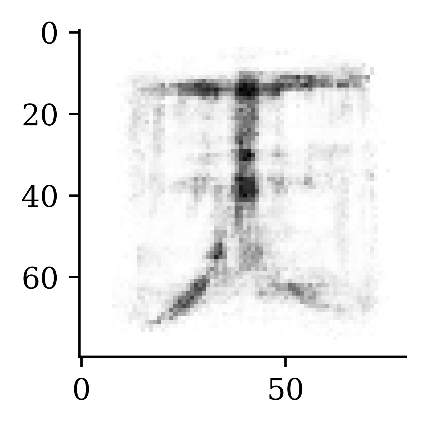

The recovered image is not as sharp as the original image, however, we can see that the high-level representation of the original picture is reconstrcuted.

Invert the images

Another way to attempt the autoencoder would be to invert the colours of the image. Following example shows, how the colours in the images are swapped. The areas which were previously in white are now in black and vice versa. The motivation behind inverting the colours is to make the input more suited for the relu activation. relu returns zeros, and zero corresponds to the black colour. If the image has more black colour, there is a chance the neural network might train more efficiently. Hence we try inverting the colours as a preprocessing before we pass it through the encoding stage.

plt.imshow(255 - X_train[0], cmap="gray");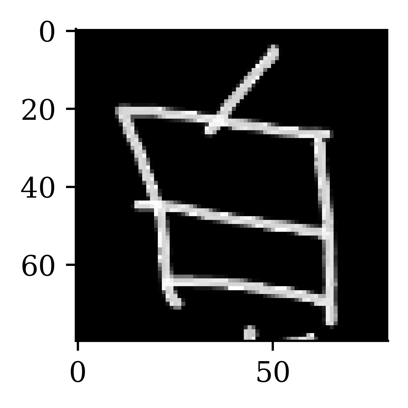

plt.imshow(255 - X_train[42], cmap="gray");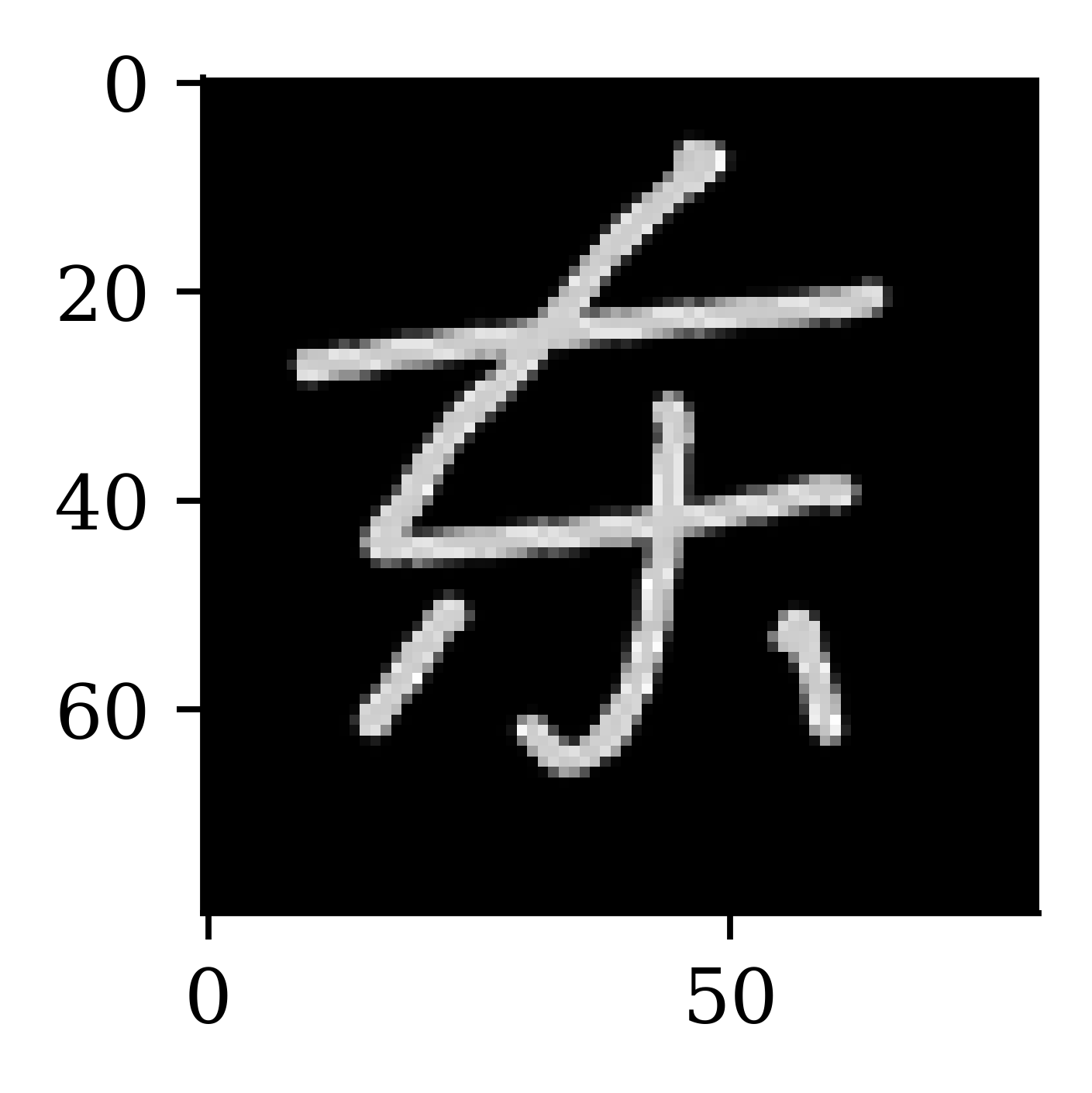

Try inverting the images

Following code shows how the same code as before is implemented, but with an additional step for inverting the pixel values of the data before parsing it through the encoding step.

random.seed(123)

model = keras.models.Sequential([
    layers.Input((img_height, img_width, 1)),
    layers.Rescaling(1./255),
1    layers.Lambda(lambda x: 1 - x),
    layers.Flatten(),
    layers.Dense(num_hidden_layer, "relu"),
    layers.Dense(img_height*img_width, "sigmoid"),
2    layers.Lambda(lambda x: 1 - x),
    layers.Reshape((img_height, img_width, 1)),
    layers.Rescaling(255),
])

model.compile("adam", "mse")
model.fit(X_train, X_train, epochs=epochs, verbose=0,
    validation_data=(X_val, X_val), callbacks=es);

1: Inverts the colours by mapping the function with x: 1-x
2: Reverses the inversion to make sure the same input image is reconstructed

The model

model.summary()

Model: "sequential_1"

┏━━━━━━━━━━━━━━━━━━━━━━━━━━━━━━━━━┳━━━━━━━━━━━━━━━━━━━━━━━━┳━━━━━━━━━━━━━━━┓
┃ Layer (type)                    ┃ Output Shape           ┃       Param # ┃
┡━━━━━━━━━━━━━━━━━━━━━━━━━━━━━━━━━╇━━━━━━━━━━━━━━━━━━━━━━━━╇━━━━━━━━━━━━━━━┩
│ rescaling_2 (Rescaling)         │ (None, 80, 80, 1)      │             0 │
├─────────────────────────────────┼────────────────────────┼───────────────┤
│ lambda (Lambda)                 │ (None, 80, 80, 1)      │             0 │
├─────────────────────────────────┼────────────────────────┼───────────────┤
│ flatten_1 (Flatten)             │ (None, 6400)           │             0 │
├─────────────────────────────────┼────────────────────────┼───────────────┤
│ dense_2 (Dense)                 │ (None, 400)            │     2,560,400 │
├─────────────────────────────────┼────────────────────────┼───────────────┤
│ dense_3 (Dense)                 │ (None, 6400)           │     2,566,400 │
├─────────────────────────────────┼────────────────────────┼───────────────┤
│ lambda_1 (Lambda)               │ (None, 6400)           │             0 │
├─────────────────────────────────┼────────────────────────┼───────────────┤
│ reshape_1 (Reshape)             │ (None, 80, 80, 1)      │             0 │
├─────────────────────────────────┼────────────────────────┼───────────────┤
│ rescaling_3 (Rescaling)         │ (None, 80, 80, 1)      │             0 │
└─────────────────────────────────┴────────────────────────┴───────────────┘

 Total params: 15,380,402 (58.67 MB)

 Trainable params: 5,126,800 (19.56 MB)

 Non-trainable params: 0 (0.00 B)

 Optimizer params: 10,253,602 (39.11 MB)

model.evaluate(X_val, X_val, verbose=0)

4181.1240234375

Some recovered image

X_val_rec = model.predict(X_val, verbose=0)

plt.imshow(X_val[42], cmap="gray");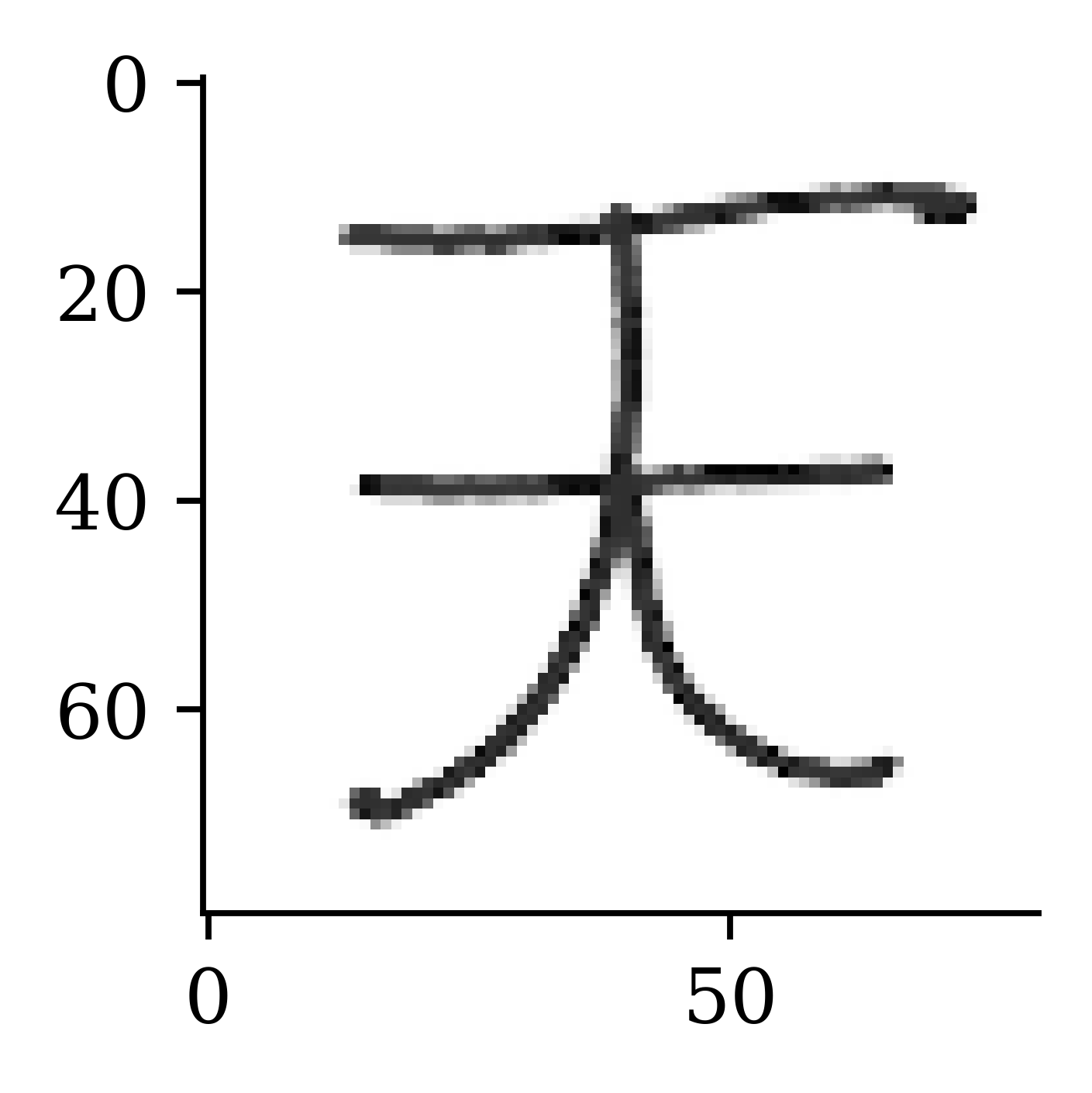

plt.imshow(X_val_rec[42], cmap="gray");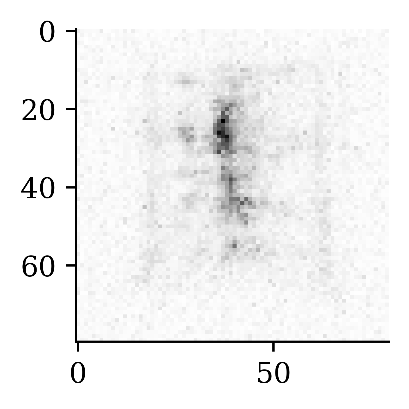

The recovered image is not too different to the image from the previous example.

CNN-enhanced encoder

To further improve the process, we can try neural networks specialized for image processing. Here we use a Convolutional Neural Network lith convolutional and pooling layers. The following example shows how we first specify the encoder, and then the decoder. The two architectures are combined at the final stage.

1random.seed(123)

2encoder = keras.models.Sequential([
    layers.Input((img_height, img_width, 1)),
3    layers.Rescaling(1./255),
4    layers.Lambda(lambda x: 1 - x),
5    layers.Conv2D(16, 3, padding="same", activation="relu"),
6    layers.MaxPooling2D(),
7    layers.Conv2D(32, 3, padding="same", activation="relu"),
    layers.MaxPooling2D(),
    layers.Conv2D(64, 3, padding="same", activation="relu"),
    layers.MaxPooling2D(),
    layers.Flatten(),
    layers.Dense(num_hidden_layer, "relu")
])

1: Sets the random seed for reproducibility
2: Starts specifying the encoder
3: Rescales the image pixel values to range between [0,1]
4: Inverts the colours of the image
5: Applies a 2D convolutional layer with 16 filters, each of size 3 \times 3, and having the same padding. same padding ensures that the output from the layer has the same heigh and width as the input
6: Performs max-pooling to reduce the dimension of the feature space
7: CNN-enhanced decoder

decoder = keras.models.Sequential([
    keras.Input(shape=(num_hidden_layer,)),
    layers.Dense(20*20),
    layers.Reshape((20, 20, 1)),
    layers.Conv2D(128, 3, padding="same", activation="relu"),
    layers.UpSampling2D(),
    layers.Conv2D(64, 3, padding="same", activation="relu"),
    layers.UpSampling2D(),
    layers.Conv2D(1, 1, padding="same", activation="relu"),
    layers.Lambda(lambda x: 1 - x),
    layers.Rescaling(255),
])

model = keras.models.Sequential([encoder, decoder])
model.compile("adam", "mse")
model.fit(X_train, X_train, epochs=epochs, verbose=0,
    validation_data=(X_val, X_val), callbacks=es);

Encoder summary

encoder.summary()

Model: "sequential_2"

┏━━━━━━━━━━━━━━━━━━━━━━━━━━━━━━━━━┳━━━━━━━━━━━━━━━━━━━━━━━━┳━━━━━━━━━━━━━━━┓
┃ Layer (type)                    ┃ Output Shape           ┃       Param # ┃
┡━━━━━━━━━━━━━━━━━━━━━━━━━━━━━━━━━╇━━━━━━━━━━━━━━━━━━━━━━━━╇━━━━━━━━━━━━━━━┩
│ rescaling_4 (Rescaling)         │ (None, 80, 80, 1)      │             0 │
├─────────────────────────────────┼────────────────────────┼───────────────┤
│ lambda_2 (Lambda)               │ (None, 80, 80, 1)      │             0 │
├─────────────────────────────────┼────────────────────────┼───────────────┤
│ conv2d (Conv2D)                 │ (None, 80, 80, 16)     │           160 │
├─────────────────────────────────┼────────────────────────┼───────────────┤
│ max_pooling2d (MaxPooling2D)    │ (None, 40, 40, 16)     │             0 │
├─────────────────────────────────┼────────────────────────┼───────────────┤
│ conv2d_1 (Conv2D)               │ (None, 40, 40, 32)     │         4,640 │
├─────────────────────────────────┼────────────────────────┼───────────────┤
│ max_pooling2d_1 (MaxPooling2D)  │ (None, 20, 20, 32)     │             0 │
├─────────────────────────────────┼────────────────────────┼───────────────┤
│ conv2d_2 (Conv2D)               │ (None, 20, 20, 64)     │        18,496 │
├─────────────────────────────────┼────────────────────────┼───────────────┤
│ max_pooling2d_2 (MaxPooling2D)  │ (None, 10, 10, 64)     │             0 │
├─────────────────────────────────┼────────────────────────┼───────────────┤
│ flatten_2 (Flatten)             │ (None, 6400)           │             0 │
├─────────────────────────────────┼────────────────────────┼───────────────┤
│ dense_4 (Dense)                 │ (None, 400)            │     2,560,400 │
└─────────────────────────────────┴────────────────────────┴───────────────┘

 Total params: 2,583,696 (9.86 MB)

 Trainable params: 2,583,696 (9.86 MB)

 Non-trainable params: 0 (0.00 B)

Decoder summary

decoder.summary()

Model: "sequential_3"

┏━━━━━━━━━━━━━━━━━━━━━━━━━━━━━━━━━┳━━━━━━━━━━━━━━━━━━━━━━━━┳━━━━━━━━━━━━━━━┓
┃ Layer (type)                    ┃ Output Shape           ┃       Param # ┃
┡━━━━━━━━━━━━━━━━━━━━━━━━━━━━━━━━━╇━━━━━━━━━━━━━━━━━━━━━━━━╇━━━━━━━━━━━━━━━┩
│ dense_5 (Dense)                 │ (None, 400)            │       160,400 │
├─────────────────────────────────┼────────────────────────┼───────────────┤
│ reshape_2 (Reshape)             │ (None, 20, 20, 1)      │             0 │
├─────────────────────────────────┼────────────────────────┼───────────────┤
│ conv2d_3 (Conv2D)               │ (None, 20, 20, 128)    │         1,280 │
├─────────────────────────────────┼────────────────────────┼───────────────┤
│ up_sampling2d (UpSampling2D)    │ (None, 40, 40, 128)    │             0 │
├─────────────────────────────────┼────────────────────────┼───────────────┤
│ conv2d_4 (Conv2D)               │ (None, 40, 40, 64)     │        73,792 │
├─────────────────────────────────┼────────────────────────┼───────────────┤
│ up_sampling2d_1 (UpSampling2D)  │ (None, 80, 80, 64)     │             0 │
├─────────────────────────────────┼────────────────────────┼───────────────┤
│ conv2d_5 (Conv2D)               │ (None, 80, 80, 1)      │            65 │
├─────────────────────────────────┼────────────────────────┼───────────────┤
│ lambda_3 (Lambda)               │ (None, 80, 80, 1)      │             0 │
├─────────────────────────────────┼────────────────────────┼───────────────┤
│ rescaling_5 (Rescaling)         │ (None, 80, 80, 1)      │             0 │
└─────────────────────────────────┴────────────────────────┴───────────────┘

 Total params: 235,537 (920.07 KB)

 Trainable params: 235,537 (920.07 KB)

 Non-trainable params: 0 (0.00 B)

model.evaluate(X_val, X_val, verbose=0)

3442.788330078125

Some recovered image

X_val_rec = model.predict(X_val, verbose=0)

plt.imshow(X_val[42], cmap="gray");

plt.imshow(X_val_rec[42], cmap="gray");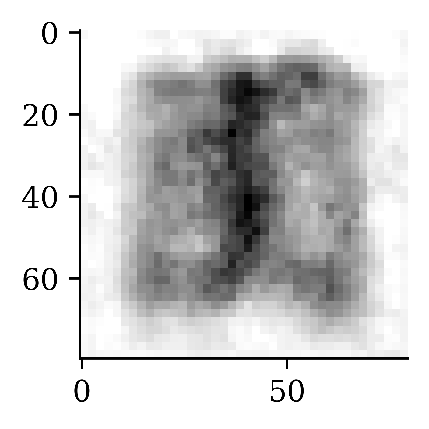

Latent space vs word embedding

We revisit the concept of word embedding, where words in the vocabulary are mapped into vector representations. Words with similar meaning should lie close to one another in the word-embedding space.
Latent space contains low-dimensional representation of data. Data/Images that are similar should lie close in the latent space.
There are pre-trained word-embedding spaces such as those for English-language movie review, German-language legal documents, etc. Semantic relationships between words differ for different tasks. Similarly, the structure of latent spaces for different data sets (humans faces, animals, etc) are different.

Latent space vs word embedding

Given a latent space of representations, or an embedding space, certain directions in the space may encode interesting axes of variation in the original data.
A concept vector is a direction of variation in the data. For example there may be a smile vector such that if z is the latent representation of a face, then z+s is the representation of the same face, smiling. We can generate an image of the person smiling from this latent representation.

Intentionally add noise to inputs

mask = rnd.random(size=X_train.shape[1:]) < 0.5
plt.imshow(mask * (255 - X_train[0]), cmap="gray");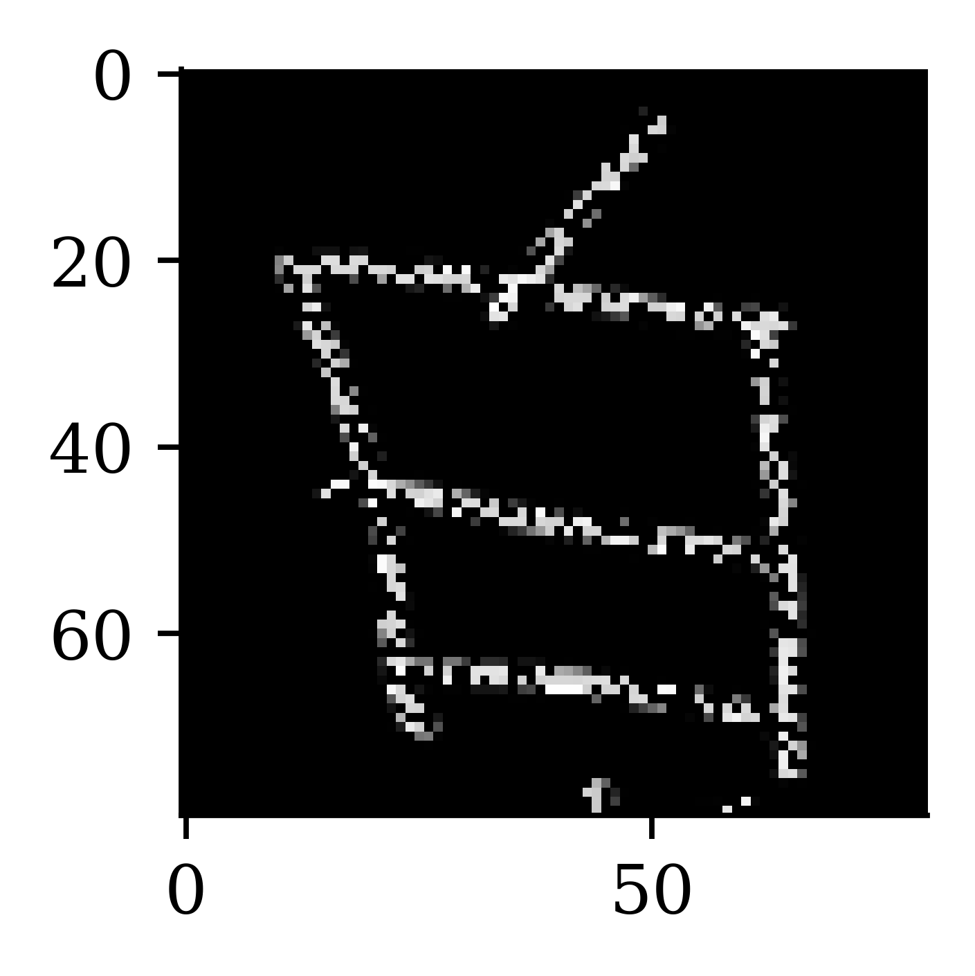

mask = rnd.random(size=X_train.shape[1:]) < 0.5
plt.imshow(mask * (255 - X_train[42]) * mask, cmap="gray");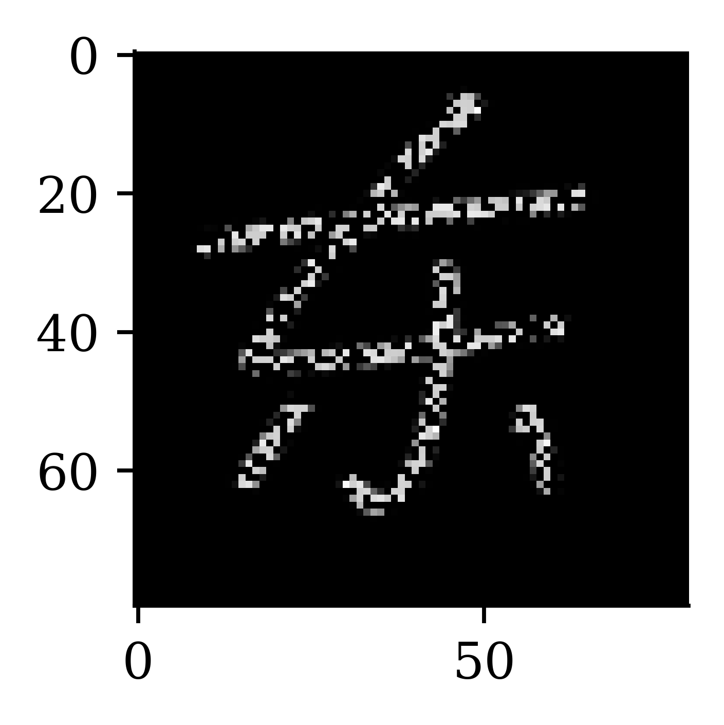

Denoising autoencoder

Can be used to do feature engineering for supervised learning problems

It is also possible to include input variables as outputs to infer missing values or just help the model “understand” the features – in fact the winning solution of a claims prediction Kaggle competition heavily used denoising autoencoders together with model stacking and ensembling – read more here.

Jacky Poon

Variational Autoencoders

Variational autoencoder

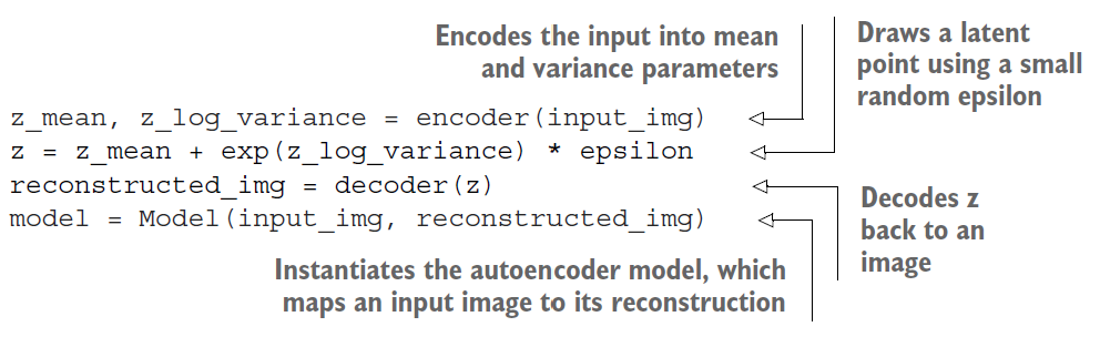
A slightly different sample from the distribution in the latent space will be decoded to a slightly different image. The stochasticity of this process improves robustness and forces the latent space to encode meaningful representation everywhere: every point in the latent space is decoded to a valid output. So the latent spaces of VAEs are continuous and highly-structured.

VAE schematic process

Focus on the decoder

Sampling new artificial images from the latent space.

Exploring the MNIST latent space

Example of MNIST-like images generated from the latent space.

Recommended Viewing

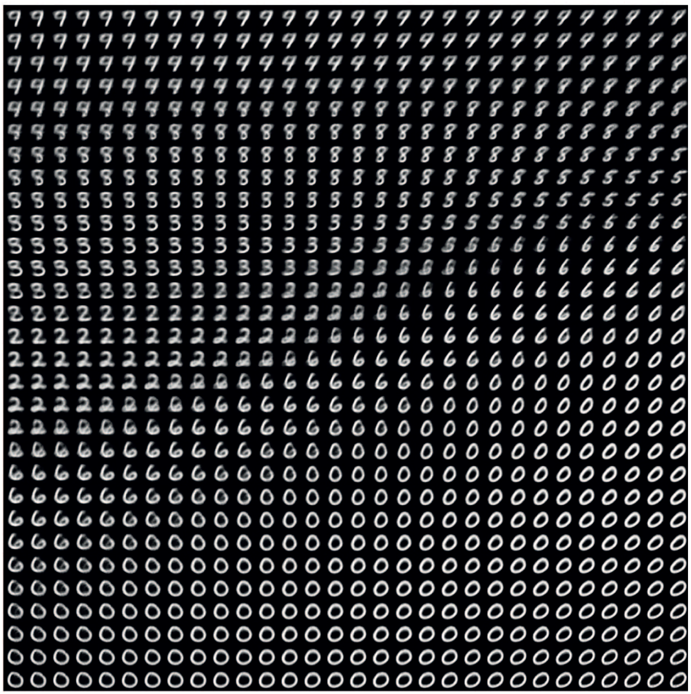
Both autoencoders and variational autoencoders aim to obtain latent representations of input data that carry same information but in a lower dimensional space. The difference between the two is that, autoencoders outputs the latent representations as vectors, while variational auto encoders first identifies the distribution of the input in the latent space, and then sample an observation from that as the vector. Autoencoders are better suited for dimensionality reduction and feature learning tasks. Variation autoencoders are better suited for generative modelling tasks and uncertainty estimation.

Diffusion Models

Using KerasCV

Package Versions

from watermark import watermark
print(watermark(python=True, packages="keras,matplotlib,numpy,pandas,seaborn,scipy,torch,tensorflow,tf_keras"))

Python implementation: CPython
Python version       : 3.11.8
IPython version      : 8.23.0

keras     : 3.2.0
matplotlib: 3.8.4
numpy     : 1.26.4
pandas    : 2.2.1
seaborn   : 0.13.2
scipy     : 1.11.0
torch     : 2.2.2
tensorflow: 2.16.1
tf_keras  : 2.16.0

Glossary

autoencoder (variational)
beam search
bias
ChatGPT (& RLHF)
DeepDream
greedy sampling

HuggingFace
language model
latent space
neural style transfer
softmax temperature
stochastic sampling

Text Generation

Generative deep learning

Text generation

Word-level language model

Character-level language model

Useful for speech recognition

Generating Shakespeare I

Generating Shakespeare II

Generating Shakespeare III

Sampling strategy

Softmax temperature

“I am a” …

Generating Laub (temp = 0.01)

Generating Laub (temp = 0.25)

Generating Laub (temp = 0.5)

Generating Laub (temp = 1)

Generating Laub (temp = 1.5)

Generate the most likely sequence

Beam search

Transformers

Transformer architecture

Transformer architecture reference

🤗 Transformers package

Reading the course profile

Question answering

ChatGPT is Transformer + RLHF

ChatGPT internals

ChatGPT

Recommended reading

Image Generation

Reverse-engineering a CNN

Adversarial examples

Adversarial stickers

Adversarial text

Deep Dream

DeepDream

DeepDream

Original

Transformed

Neural style transfer

Neural style transfer

Goal of NST

A wanderer in Greenland

A wanderer in Greenland II

A new style image

A new content image

Another neural style transfer

Why is this important?

Autoencoders

Autoencoder

Autoencoder II

Example: PSAM

A compression game

Make a basic autoencoder

The model

Some recovered image

Invert the images

Try inverting the images

The model

Some recovered image

CNN-enhanced encoder

Encoder summary

Decoder summary

Some recovered image

Latent space vs word embedding

Latent space vs word embedding

Intentionally add noise to inputs

Denoising autoencoder

Variational Autoencoders

Variational autoencoder

VAE schematic process

Focus on the decoder

Exploring the MNIST latent space

Recommended Viewing

Diffusion Models

Using KerasCV

Package Versions

Glossary