Classification

ACTL3143 & ACTL5111 Deep Learning for Actuaries

Author

Patrick Laub

Show the package imports
import random
import matplotlib.pyplot as plt
import numpy as np
import pandas as pd
import seaborn as sns

from keras.models import Sequential
from keras.layers import Dense, Input
from keras.callbacks import EarlyStopping

from sklearn.model_selection import train_test_split
from sklearn.preprocessing import OneHotEncoder, StandardScaler
from sklearn.compose import make_column_transformer
from sklearn.impute import SimpleImputer
from sklearn import set_config

set_config(transform_output="pandas")

Classification

Iris dataset

from sklearn.datasets import load_iris
iris = load_iris()
names = ["SepalLength", "SepalWidth", "PetalLength", "PetalWidth"]
features = pd.DataFrame(iris.data, columns = names)
features
SepalLength SepalWidth PetalLength PetalWidth
0 5.1 3.5 1.4 0.2
1 4.9 3.0 1.4 0.2
... ... ... ... ...
148 6.2 3.4 5.4 2.3
149 5.9 3.0 5.1 1.8

150 rows × 4 columns

Target variable

iris.target_names
array(['setosa', 'versicolor', 'virginica'], dtype='<U10')
iris.target[:8]
array([0, 0, 0, 0, 0, 0, 0, 0])
target = iris.target
target = target.reshape(-1, 1)
target[:8]
array([[0],
       [0],
       [0],
       [0],
       [0],
       [0],
       [0],
       [0]])
classes, counts = np.unique(
        target,
        return_counts=True
)
print(classes)
print(counts)
[0 1 2]
[50 50 50]
iris.target_names[
  target[[0, 30, 60]]
]
array([['setosa'],
       ['setosa'],
       ['versicolor']], dtype='<U10')

Split the data into train and test

X_train, X_test, y_train, y_test = train_test_split(features, target, random_state=24)
X_train
SepalLength SepalWidth PetalLength PetalWidth
53 5.5 2.3 4.0 1.3
58 6.6 2.9 4.6 1.3
95 5.7 3.0 4.2 1.2
... ... ... ... ...
145 6.7 3.0 5.2 2.3
87 6.3 2.3 4.4 1.3
131 7.9 3.8 6.4 2.0

112 rows × 4 columns

X_test.shape, y_test.shape
((38, 4), (38, 1))

A basic classifier network

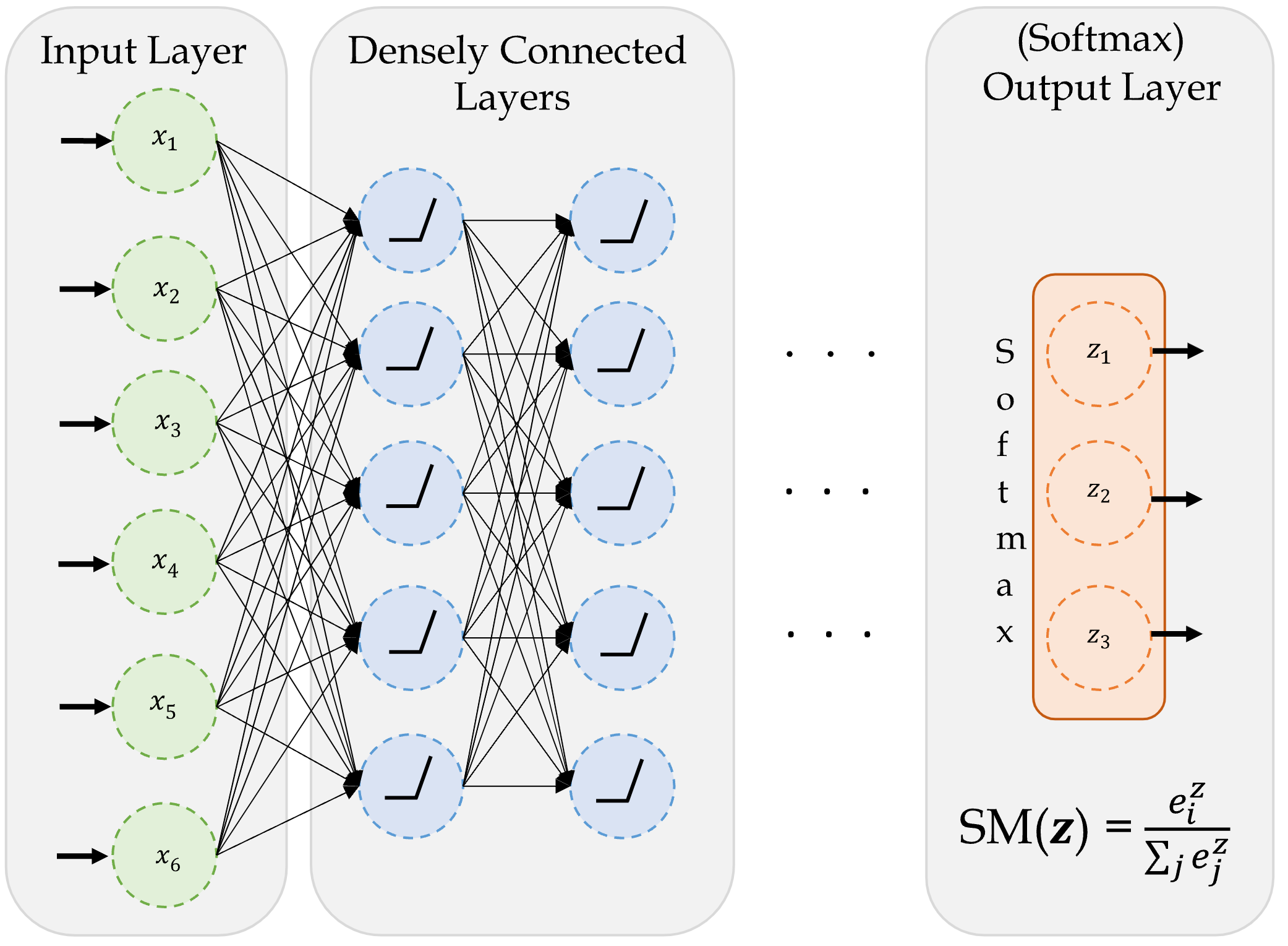
A basic network for classifying into three categories.

Since the task is a classification problem, we use softmax activation function. The softmax function takes in the input and returns a probability vector, which tells us about the probability of a data point belonging to a certain class.

Create a classifier model

NUM_FEATURES = len(features.columns)
NUM_CATS = len(np.unique(target))

print("Number of features:", NUM_FEATURES)
print("Number of categories:", NUM_CATS)
Number of features: 4
Number of categories: 3

Make a function to return a Keras model:

def build_model(seed=42):
    random.seed(seed)
    return Sequential([
        Dense(30, activation="relu"),
        Dense(NUM_CATS, activation="softmax")
    ])

Fit the model

model = build_model()
model.compile("adam", "sparse_categorical_crossentropy")

model.fit(X_train, y_train, epochs=5, verbose=2);
Epoch 1/5
4/4 - 0s - 2ms/step - loss: 1.3870
Epoch 2/5
4/4 - 0s - 1ms/step - loss: 1.2943
Epoch 3/5
4/4 - 0s - 1ms/step - loss: 1.2189
Epoch 4/5
4/4 - 0s - 1ms/step - loss: 1.1581
Epoch 5/5
4/4 - 0s - 1ms/step - loss: 1.1079

Since the problem at hand is a classification problem, we define the optimizer and loss function accordingly. Optimizer is adam and the loss function is sparse_categorical_crossentropy. If the response variable represents the category directly using an integer (i.e. if the response variable is not one-hot encoded), we must use sparse_categorical_crossentropy. If the response variable (y label) is already one-hot encoded we can use categorical_crossentropy.

Track accuracy as the model trains

model = build_model()
model.compile("adam", "sparse_categorical_crossentropy", \
        metrics=["accuracy"])
model.fit(X_train, y_train, epochs=5, verbose=2);
Epoch 1/5
4/4 - 0s - 1ms/step - accuracy: 0.2857 - loss: 1.3923
Epoch 2/5
4/4 - 0s - 1ms/step - accuracy: 0.2857 - loss: 1.2910
Epoch 3/5
4/4 - 0s - 1ms/step - accuracy: 0.2857 - loss: 1.2179
Epoch 4/5
4/4 - 0s - 1ms/step - accuracy: 0.3036 - loss: 1.1603
Epoch 5/5
4/4 - 0s - 1ms/step - accuracy: 0.4286 - loss: 1.1095

We can also specify which loss metric to monitor in assessing the performance during the training. The metric that is usually used in classification tasks is accuracy, which tracks the fraction of all predictions which identified the class accurately. The metrics are not used for optimizing. They are only used to keep track of how well the model is performing during the optimization. By setting verbose=2, we are printing the progress during training, and we can see how the loss is reducing and accuracy is improving.

Run a long fit

Run the model training for 500 epochs.

model = build_model()
model.compile("adam", "sparse_categorical_crossentropy", \
        metrics=["accuracy"])
%time hist = model.fit(X_train, y_train, epochs=500, \
        validation_split=0.25, verbose=False)
CPU times: user 1.91 s, sys: 1.88 ms, total: 1.91 s
Wall time: 1.92 s

Evaluation now returns both loss and accuracy.

model.evaluate(X_test, y_test, verbose=False)
[0.08759287744760513, 0.9736841917037964]

Add early stopping

model = build_model()
model.compile("adam", "sparse_categorical_crossentropy", \
        metrics=["accuracy"])

es = EarlyStopping(restore_best_weights=True, patience=50,
        monitor="val_accuracy")                                         
%time hist_es = model.fit(X_train, y_train, epochs=500, \
        validation_split=0.25, callbacks=[es], verbose=False);

print(f"Stopped after {len(hist_es.history['loss'])} epochs.")
CPU times: user 280 ms, sys: 791 µs, total: 281 ms
Wall time: 282 ms
Stopped after 68 epochs.
  1. Defines a new model with the same architecture as model_build which is already constructed
  2. Compiles the model with optimizer, loss function and metric
  3. Defines the early stopping object as usual, with one slight change. The code is specified to activate the early stopping by monitoring the validation accuracy (val_accuracy), not the loss.
  4. Fits the model

Evaluation on test set:

model.evaluate(X_test, y_test, verbose=False)
[0.8151808977127075, 0.9473684430122375]
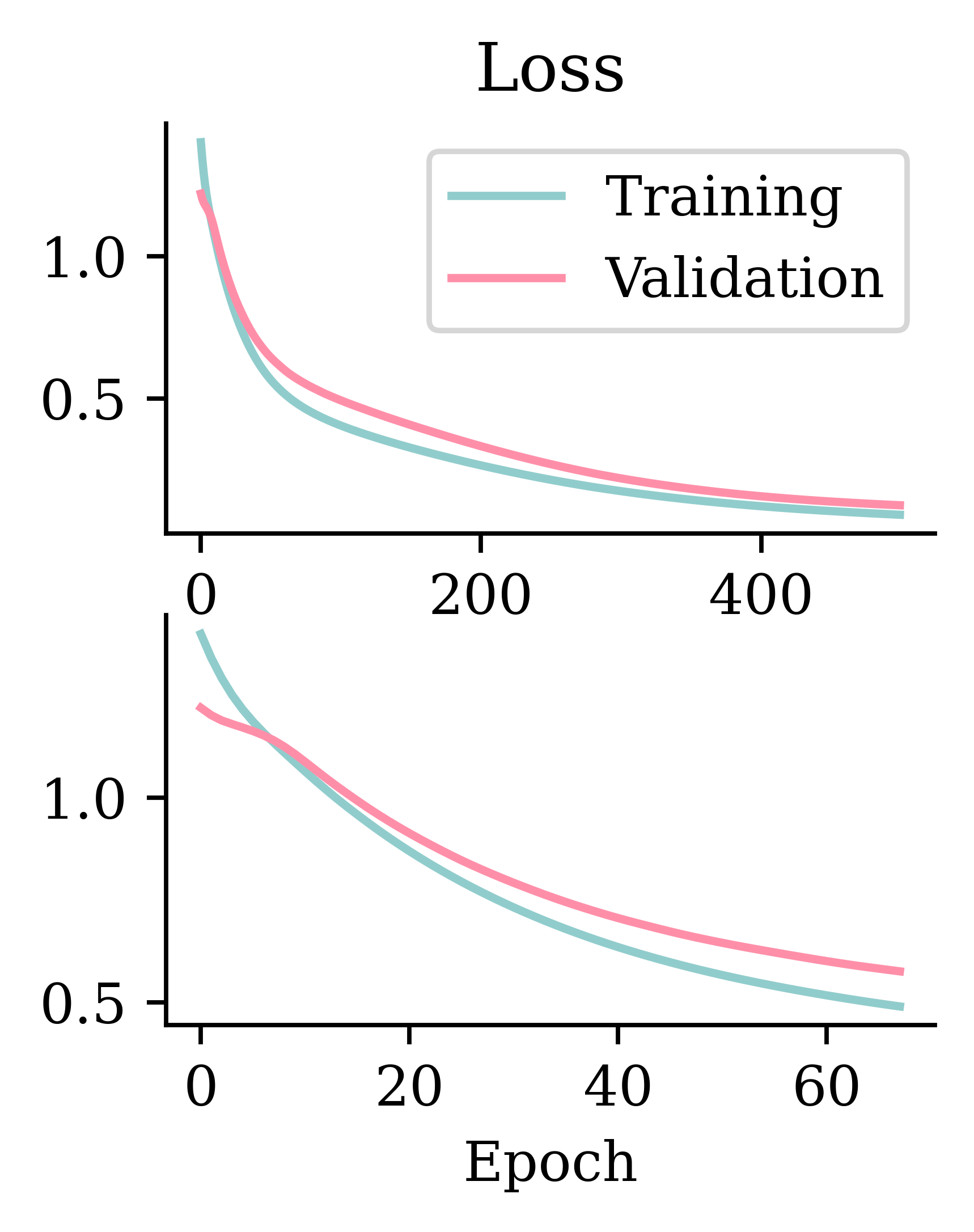
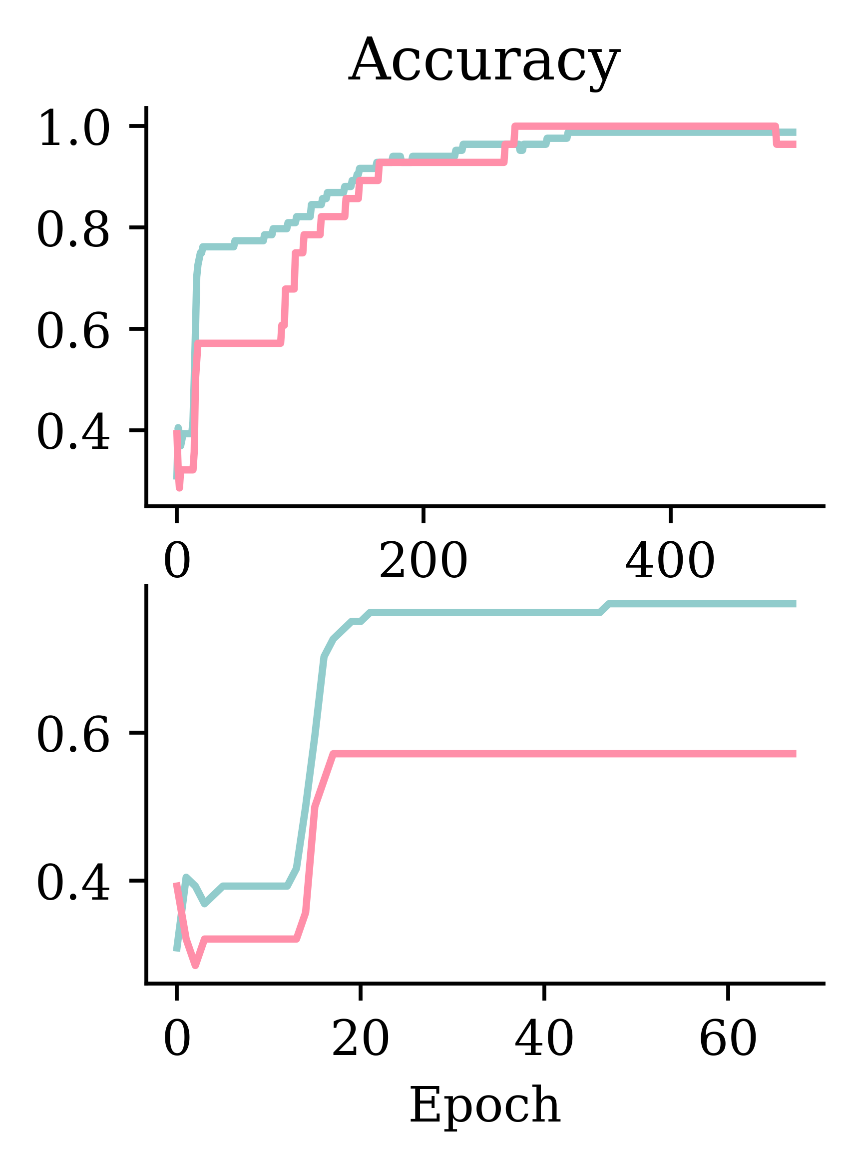
Fitting metrics

Left hand side plots show how loss behaved without and with early stopping. Right hand side plots show how accuracy performed without and with early stopping.

What is the softmax activation?

It creates a “probability” vector: \text{Softmax}(\boldsymbol{x}) = \frac{\mathrm{e}^x_i}{\sum_j \mathrm{e}^x_j} \,.

In NumPy:

out = np.array([5, -1, 6])
(np.exp(out) / np.exp(out).sum()).round(3)
array([0.269, 0.001, 0.731])

In Keras:

out = keras.ops.convert_to_tensor([[5.0, -1.0, 6.0]])
keras.ops.round(keras.ops.softmax(out), 3)
tensor([[0.2690, 0.0010, 0.7310]])

Prediction using classifiers

y_test[:4]
array([[2],
       [2],
       [1],
       [1]])

The response variable y is an array of numeric integers, each representing a class to which the data belongs. However, the model.predict() function returns an array with probabilities not an array with integers. The array displays the probabilities of belonging to each category.
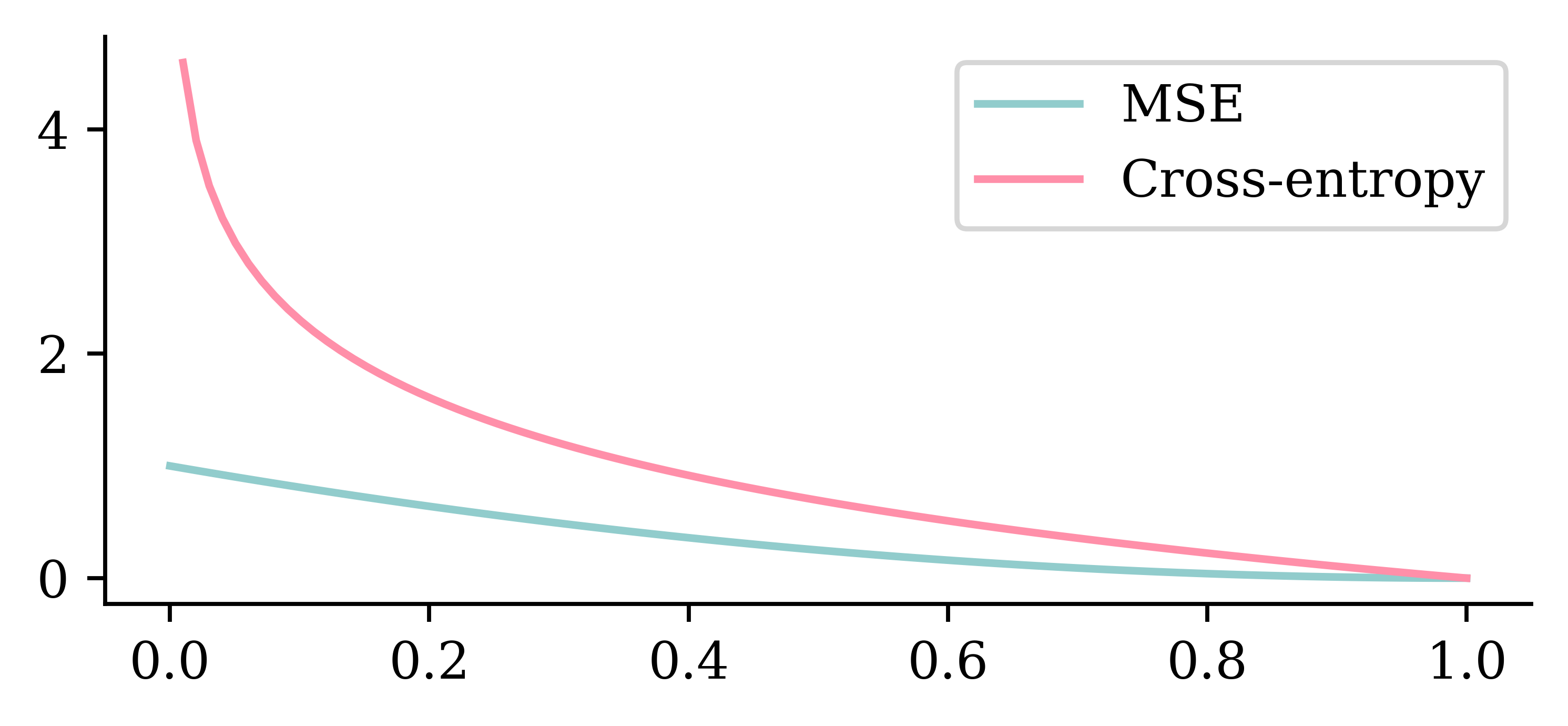
y_pred = model.predict(X_test.head(4), verbose=0)
y_pred
array([[0.16517346, 0.41306466, 0.4217618 ],
       [0.1688867 , 0.3096904 , 0.5214229 ],
       [0.279566  , 0.4134798 , 0.30695418],
       [0.2462524 , 0.38838378, 0.3653639 ]], dtype=float32)

Using np.argmax() which returns index of the maximum value in an array, we can obtain the predicted class.

# Add 'keepdims=True' to get a column vector.
np.argmax(y_pred, axis=1)
array([2, 2, 1, 1])
iris.target_names[np.argmax(y_pred, axis=1)]
array(['virginica', 'virginica', 'versicolor', 'versicolor'], dtype='<U10')

Cross-entropy loss: ELI5

Why use cross-entropy loss?

p = np.linspace(0, 1, 100)
plt.plot(p, (1-p)**2)
plt.plot(p, -np.log(p))
plt.legend(["MSE", "Cross-entropy"]);
/var/folders/sq/__n07d014s3gvhj5fy8b61zr0000gn/T/ipykernel_37011/2228567616.py:3: RuntimeWarning: divide by zero encountered in log
  plt.plot(p, -np.log(p))

The above plot shows how MSE and cross-entropy penalize wrong predictions. The x-axis indicates the severity of misclassification. Suppose the neural network predicted that there is near-zero probability of an observation being in class “1” when the actual class is “1”. This represents a strong misclassification. The above graph shows how MSE does not impose heavy penalties for the misclassifications near zero. It displays a linear increment across the severity of misclassification. On the other hand, cross-entropy penalises bad predictions strongly. Also, the misclassification penalty grows exponentially. This makes cross entropy more suitable.

One-hot encoding

from sklearn.preprocessing import OneHotEncoder

enc = OneHotEncoder(sparse_output=False)

y_train_oh = enc.fit_transform(y_train)
y_test_oh = enc.transform(y_test)
y_train[:5]
array([[1],
       [1],
       [1],
       [0],
       [0]])
y_train_oh[:5]
x0_0 x0_1 x0_2
0 0.0 1.0 0.0
1 0.0 1.0 0.0
2 0.0 1.0 0.0
3 1.0 0.0 0.0
4 1.0 0.0 0.0

Classifier given one-hot outputs

Create the model (new loss function):

model = build_model()
model.compile("adam", "categorical_crossentropy", \
    metrics=["accuracy"])

Fit the model (new target variables):

model.fit(X_train, y_train_oh, epochs=100, verbose=False);

Evaluate the model (new target variables):

model.evaluate(X_test, y_test_oh, verbose=False)
[0.29025211930274963, 0.9473684430122375]

Stroke Prediction

The data

Dataset source: Kaggle Stroke Prediction Dataset.

data = pd.read_csv("stroke.csv")
data.head()
id gender age hypertension heart_disease ever_married work_type Residence_type avg_glucose_level bmi smoking_status stroke
0 9046 Male 67.0 0 1 Yes Private Urban 228.69 36.6 formerly smoked 1
1 51676 Female 61.0 0 0 Yes Self-employed Rural 202.21 NaN never smoked 1
2 31112 Male 80.0 0 1 Yes Private Rural 105.92 32.5 never smoked 1
3 60182 Female 49.0 0 0 Yes Private Urban 171.23 34.4 smokes 1
4 1665 Female 79.0 1 0 Yes Self-employed Rural 174.12 24.0 never smoked 1

Data description

  1. id: unique identifier
  2. gender: “Male”, “Female” or “Other”
  3. age: age of the patient
  4. hypertension: 0 or 1 if the patient has hypertension
  5. heart_disease: 0 or 1 if the patient has any heart disease
  6. ever_married: “No” or “Yes”
  7. work_type: “children”, “Govt_jov”, “Never_worked”, “Private” or “Self-employed”
  1. Residence_type: “Rural” or “Urban”
  2. avg_glucose_level: average glucose level in blood
  3. bmi: body mass index
  4. smoking_status: “formerly smoked”, “never smoked”, “smokes” or “Unknown”
  5. stroke: 0 or 1 if the patient had a stroke

Split the data

First, look for missing values.

number_missing = data.isna().sum()
number_missing[number_missing > 0]
bmi    201
dtype: int64
features = data.drop(["id", "stroke"], axis=1)
target = data["stroke"]

X_main, X_test, y_main, y_test = train_test_split(
    features, target, test_size=0.2, random_state=7)
X_train, X_val, y_train, y_val = train_test_split(
    X_main, y_main, test_size=0.25, random_state=12)

X_train.shape, X_val.shape, X_test.shape
((3066, 10), (1022, 10), (1022, 10))

What values do we see in the data?

X_train["gender"].value_counts()
gender
Female    1802
Male      1264
Name: count, dtype: int64
X_train["ever_married"].value_counts()
ever_married
Yes    2007
No     1059
Name: count, dtype: int64
X_train["Residence_type"].value_counts()
Residence_type
Urban    1536
Rural    1530
Name: count, dtype: int64
X_train["work_type"].value_counts()
work_type
Private          1754
Self-employed     490
children          419
Govt_job          390
Never_worked       13
Name: count, dtype: int64
X_train["smoking_status"].value_counts()
smoking_status
never smoked       1130
Unknown             944
formerly smoked     522
smokes              470
Name: count, dtype: int64

Preprocess columns individually

  1. Take categorical columns \hookrightarrow one-hot vectors
  2. binary columns \hookrightarrow do nothing
  3. continuous columns \hookrightarrow impute NaNs & standardise.

Scikit-learn column transformer

from sklearn.pipeline import make_pipeline

cat_vars =  ["gender", "ever_married", "Residence_type",
    "work_type", "smoking_status"]                  

ct = make_column_transformer(
  (OneHotEncoder(sparse_output=False, handle_unknown="ignore"), cat_vars),
  ("passthrough", ["hypertension", "heart_disease"]),
  remainder=make_pipeline(SimpleImputer(), StandardScaler()),
  verbose_feature_names_out=False
)

X_train_ct = ct.fit_transform(X_train)
X_val_ct = ct.transform(X_val)
X_test_ct = ct.transform(X_test)

for name, X in zip(("train", "val", "test"), (X_train_ct, X_val_ct, X_test_ct)):
    num_na = X.isna().sum().sum()
    print(f"The {name} set has shape {X_train_ct.shape} & with {num_na} NAs.")
The train set has shape (3066, 20) & with 0 NAs.
The val set has shape (3066, 20) & with 0 NAs.
The test set has shape (3066, 20) & with 0 NAs.
  1. Imports make_pipeline class from sklearn.pipeline library. make_pipeline is used to streamline the data pre processing. In the above example, make_pipeline is used to first treat for missing values and then scale numerical values
  2. Stores categorical variables in cat_vars
  3. Specifies the one-hot encoding for all categorical variables. We set the sparse_output=False, to return a dense array rather than a sparse matrix. handle_unknown specifies how the neural network should handle unseen categories. By setting handle_unknown="ignore", we instruct the neural network to ignore categories that were not seen during training. If we did not do this, it will interrupt the model’s operation after deployment
  4. Passes through hypertension and heart_disease without any pre processing
  5. Makes a pipeline that first applies SimpleImputer() to replace missing values with the mean and then applies StandardScaler() to scale the numerical values
  6. Prints out the missing values to ensure the SimpleImputer() has worked

Handling unseen categories

X_train["gender"].value_counts()
gender
Female    1802
Male      1264
Name: count, dtype: int64
X_val["gender"].value_counts()
gender
Female    615
Male      406
Other       1
Name: count, dtype: int64

Because the way train and test was split, one-hot encoder could not pick up on the third category. This could interrupt the model performance. To avoid such confusions, we could either give instructions manually on how to tackle unseen categories. An example is given below.

ind = np.argmax(X_val["gender"] == "Other")
X_val.iloc[ind-1:ind+3][["gender"]]
gender
4970 Male
3116 Other
4140 Male
2505 Female
gender_cols = X_val_ct[["gender_Female", "gender_Male"]]
gender_cols.iloc[ind-1:ind+3]
gender_Female gender_Male
4970 0.0 1.0
3116 0.0 0.0
4140 0.0 1.0
2505 1.0 0.0

However, to give such instructions on handling unseen categories, we would first have to know what those possible categories could be. We should also have specific knowledge on what value to assign in case they come up during model performance. One easy way to tackle it would be to use handle_unknown="ignore" during encoding, as mentioned before.

Setup a binary classification model

def create_model(seed=42):
    random.seed(seed)
    model = Sequential()
    model.add(Input(X_train_ct.shape[1:]))
    model.add(Dense(32, "leaky_relu"))
    model.add(Dense(16, "leaky_relu"))
    model.add(Dense(1, "sigmoid"))
    return model

Since this is a binary classification problem, we use the sigmoid activation function.

model = create_model()
model.summary()
Model: "sequential_5"
┏━━━━━━━━━━━━━━━━━━━━━━━━━━━━━━━━━┳━━━━━━━━━━━━━━━━━━━━━━━━┳━━━━━━━━━━━━━━━┓
┃ Layer (type)                     Output Shape                  Param # ┃
┡━━━━━━━━━━━━━━━━━━━━━━━━━━━━━━━━━╇━━━━━━━━━━━━━━━━━━━━━━━━╇━━━━━━━━━━━━━━━┩
│ dense_10 (Dense)                │ (None, 32)             │           672 │
├─────────────────────────────────┼────────────────────────┼───────────────┤
│ dense_11 (Dense)                │ (None, 16)             │           528 │
├─────────────────────────────────┼────────────────────────┼───────────────┤
│ dense_12 (Dense)                │ (None, 1)              │            17 │
└─────────────────────────────────┴────────────────────────┴───────────────┘
 Total params: 1,217 (4.75 KB)
 Trainable params: 1,217 (4.75 KB)
 Non-trainable params: 0 (0.00 B)

model.summary() returns the summary of the constructed neural network.

Add metrics, compile, and fit

model = create_model()

pr_auc = keras.metrics.AUC(curve="PR", name="pr_auc")
model.compile(optimizer="adam", loss="binary_crossentropy",
    metrics=[pr_auc, "accuracy", "auc"])                                

es = EarlyStopping(patience=50, restore_best_weights=True,
    monitor="val_pr_auc", verbose=1)
model.fit(X_train_ct, y_train, callbacks=[es], epochs=1_000, verbose=0,
  validation_data=(X_val_ct, y_val));
Epoch 69: early stopping
Restoring model weights from the end of the best epoch: 19.
  1. Brings in the created model
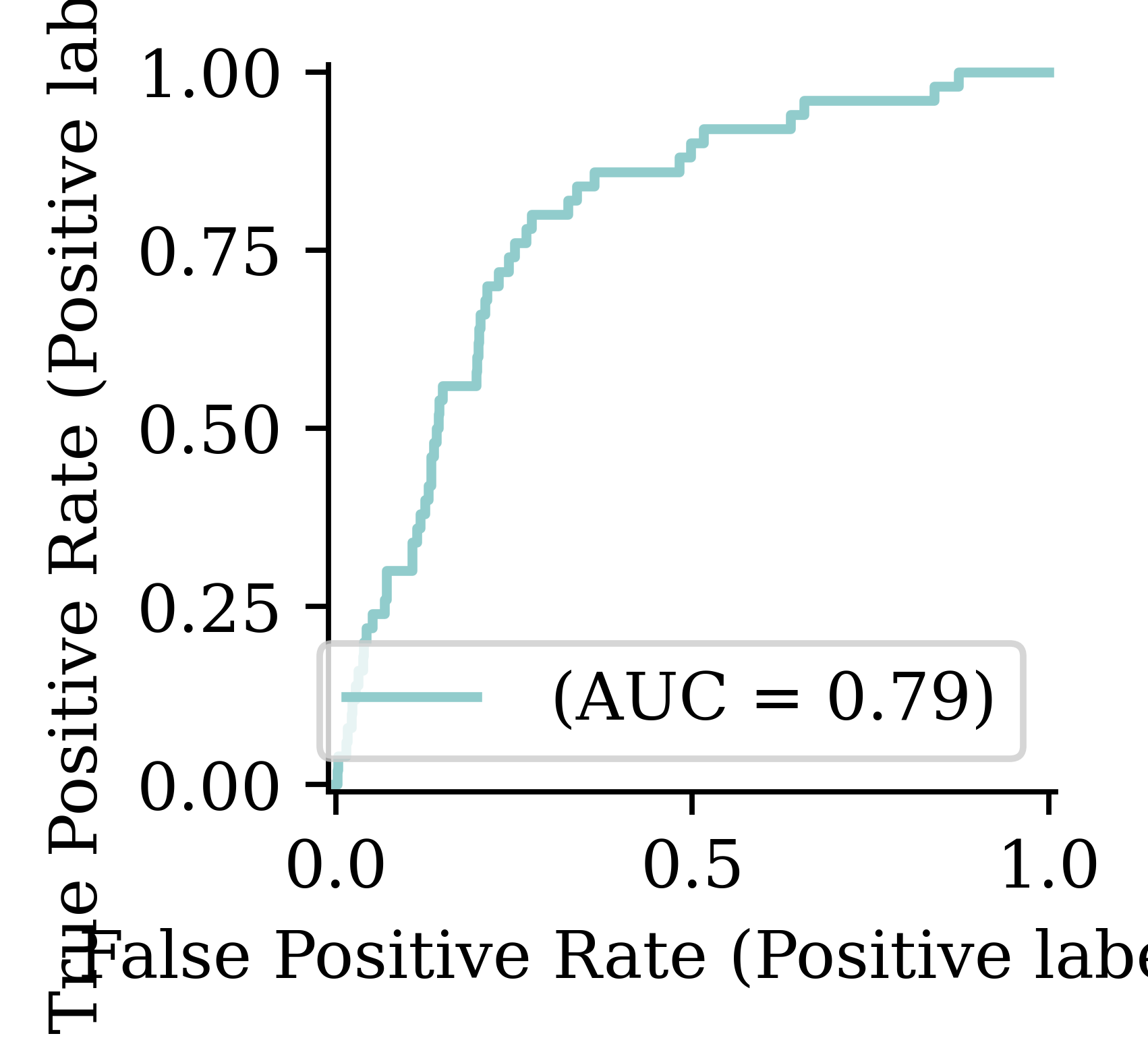
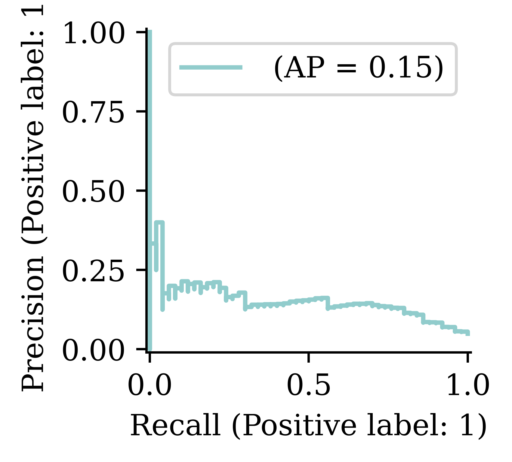
  2. Creates an instance pr_auc to store the AUC (Area Under Curve) metric for the PR (Precision-Recall) curve
  3. Compiles the model with an appropriate loss function, optimizer and relevant metrics. Since the above problem is a binary classification, we would optimize the binary_crossentropy, chose to monitor both accuracy and AUC and pr_auc.

Tracking AUC and pr_auc on top of the accuracy is important, particularly in the cases where there is a class imbalance. Suppose a data has 95% True class and only 5% False class, then, even a random classifier that predicts True 95% of the time will have a high accuracy. To avoid such issues, it is advisable to monitor both accuracy and AUC.

model.evaluate(X_val_ct, y_val, verbose=0)
[0.1450638473033905,
 0.13280197978019714,
 0.9589040875434875,
 0.8276846408843994]

Overweight the minority class

model = create_model()

pr_auc = keras.metrics.AUC(curve="PR", name="pr_auc")
model.compile(optimizer="adam", loss="binary_crossentropy",
    metrics=[pr_auc, "accuracy", "auc"])

es = EarlyStopping(patience=50, restore_best_weights=True,
    monitor="val_pr_auc", verbose=1)
model.fit(X_train_ct, y_train.to_numpy(), callbacks=[es], epochs=1_000, verbose=0,
  validation_data=(X_val_ct, y_val), class_weight={0: 1, 1: 10});
Epoch 56: early stopping
Restoring model weights from the end of the best epoch: 6.

Another way to treat class imbalance would be to assign a higher weight to the minority class during model fitting. 1. Fits the model by assigning a higher weight to the misclassification in the minor class. This above class weight assignment says that misclassifying an observation from class 1 will be penalized 10 times more than misclassifying an observation from class 0. The weights can be assigned in relation to the level of data imbalance.

model.evaluate(X_val_ct, y_val, verbose=0)
[0.379545658826828, 0.1360630989074707, 0.767123281955719, 0.8222789168357849]
model.evaluate(X_test_ct, y_test, verbose=0)
[0.3905954957008362,
 0.15662002563476562,
 0.7837573289871216,
 0.8110082149505615]

Classification Metrics

from sklearn.metrics import confusion_matrix, RocCurveDisplay, PrecisionRecallDisplay
y_pred = model.predict(X_test_ct, verbose=0)
RocCurveDisplay.from_predictions(y_test, y_pred, name="");

PrecisionRecallDisplay.from_predictions(y_test, y_pred, name=""); plt.legend(loc="upper right");

y_pred_stroke = y_pred > 0.5
confusion_matrix(y_test, y_pred_stroke)
array([[762, 210],
       [ 11,  39]])
y_pred_stroke = y_pred > 0.3
confusion_matrix(y_test, y_pred_stroke)
array([[629, 343],
       [  6,  44]])

Package Versions

from watermark import watermark
print(watermark(python=True, packages="keras,matplotlib,numpy,pandas,seaborn,scipy,torch,tensorflow,tf_keras"))
Python implementation: CPython
Python version       : 3.11.8
IPython version      : 8.23.0

keras     : 3.2.0
matplotlib: 3.8.4
numpy     : 1.26.4
pandas    : 2.2.1
seaborn   : 0.13.2
scipy     : 1.11.0
torch     : 2.2.2
tensorflow: 2.16.1
tf_keras  : 2.16.0

Glossary

  • classification problem
  • confusion matrix
  • cross-entropy loss
  • sigmoid activation function