Classification

ACTL3143 & ACTL5111 Deep Learning for Actuaries

Patrick Laub

Classification

Lecture Outline

  • Classification

  • Stroke Prediction

Iris dataset

from sklearn.datasets import load_iris
iris = load_iris()
names = ["SepalLength", "SepalWidth", "PetalLength", "PetalWidth"]
features = pd.DataFrame(iris.data, columns = names)
features
SepalLength SepalWidth PetalLength PetalWidth
0 5.1 3.5 1.4 0.2
1 4.9 3.0 1.4 0.2
... ... ... ... ...
148 6.2 3.4 5.4 2.3
149 5.9 3.0 5.1 1.8

150 rows × 4 columns

Target variable

iris.target_names
array(['setosa', 'versicolor', 'virginica'], dtype='<U10')
iris.target[:8]
array([0, 0, 0, 0, 0, 0, 0, 0])
target = iris.target
target = target.reshape(-1, 1)
target[:8]
array([[0],
       [0],
       [0],
       [0],
       [0],
       [0],
       [0],
       [0]])
classes, counts = np.unique(
        target,
        return_counts=True
)
print(classes)
print(counts)
[0 1 2]
[50 50 50]
iris.target_names[
  target[[0, 30, 60]]
]
array([['setosa'],
       ['setosa'],
       ['versicolor']], dtype='<U10')

Split the data into train and test

X_train, X_test, y_train, y_test = train_test_split(features, target, random_state=24)
X_train
SepalLength SepalWidth PetalLength PetalWidth
53 5.5 2.3 4.0 1.3
58 6.6 2.9 4.6 1.3
95 5.7 3.0 4.2 1.2
... ... ... ... ...
145 6.7 3.0 5.2 2.3
87 6.3 2.3 4.4 1.3
131 7.9 3.8 6.4 2.0

112 rows × 4 columns

X_test.shape, y_test.shape
((38, 4), (38, 1))

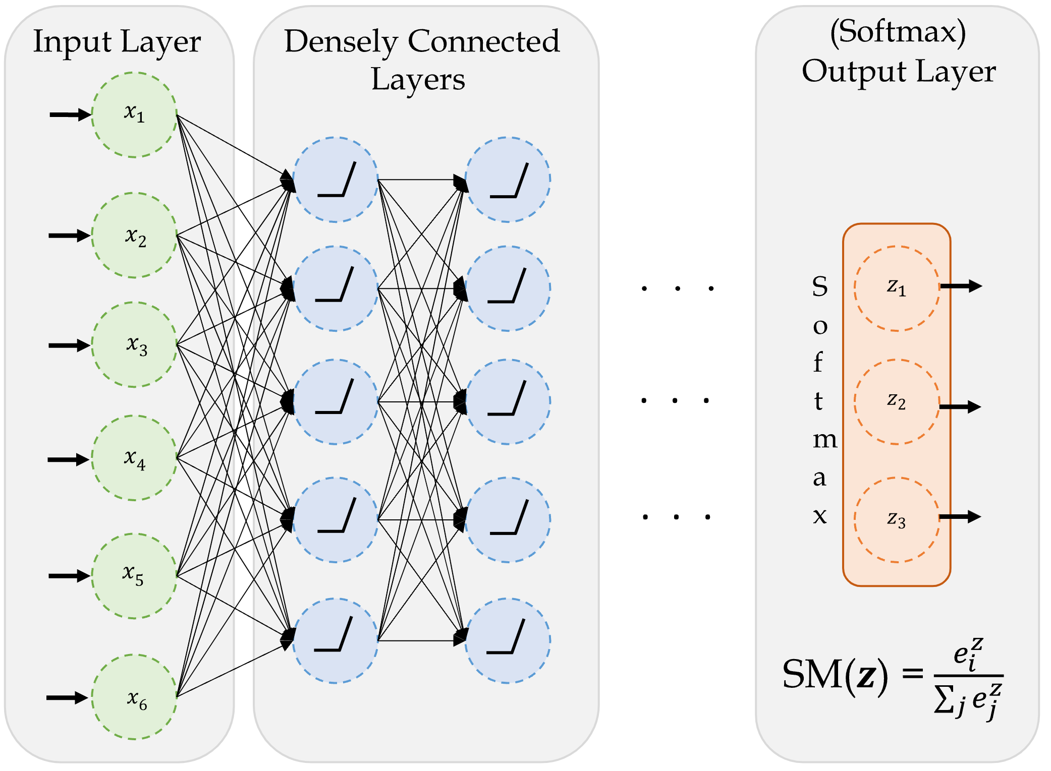
A basic classifier network

A basic network for classifying into three categories.

Create a classifier model

NUM_FEATURES = len(features.columns)
NUM_CATS = len(np.unique(target))

print("Number of features:", NUM_FEATURES)
print("Number of categories:", NUM_CATS)
Number of features: 4
Number of categories: 3

Make a function to return a Keras model:

def build_model(seed=42):
    random.seed(seed)
    return Sequential([
        Dense(30, activation="relu"),
        Dense(NUM_CATS, activation="softmax")
    ])

Fit the model

model = build_model()
model.compile("adam", "sparse_categorical_crossentropy")

model.fit(X_train, y_train, epochs=5, verbose=2);
Epoch 1/5
4/4 - 0s - 123ms/step - loss: 1.3502
Epoch 2/5
4/4 - 0s - 4ms/step - loss: 1.2852
Epoch 3/5
4/4 - 0s - 5ms/step - loss: 1.2337
Epoch 4/5
4/4 - 0s - 4ms/step - loss: 1.1915
Epoch 5/5
4/4 - 0s - 4ms/step - loss: 1.1556

Track accuracy as the model trains

model = build_model()
model.compile("adam", "sparse_categorical_crossentropy", \
        metrics=["accuracy"])
model.fit(X_train, y_train, epochs=5, verbose=2);
Epoch 1/5
4/4 - 1s - 137ms/step - accuracy: 0.2946 - loss: 1.3502
Epoch 2/5
4/4 - 0s - 5ms/step - accuracy: 0.3036 - loss: 1.2852
Epoch 3/5
4/4 - 0s - 6ms/step - accuracy: 0.3036 - loss: 1.2337
Epoch 4/5
4/4 - 0s - 15ms/step - accuracy: 0.3304 - loss: 1.1915
Epoch 5/5
4/4 - 0s - 5ms/step - accuracy: 0.3393 - loss: 1.1556

Run a long fit

model = build_model()
model.compile("adam", "sparse_categorical_crossentropy", \
        metrics=["accuracy"])
%time hist = model.fit(X_train, y_train, epochs=500, \
        validation_split=0.25, verbose=False)
CPU times: user 17.7 s, sys: 2.17 s, total: 19.9 s
Wall time: 17.9 s

Evaluation now returns both loss and accuracy.

model.evaluate(X_test, y_test, verbose=False)
[0.09586220979690552, 0.9736841917037964]

Add early stopping

model = build_model()
model.compile("adam", "sparse_categorical_crossentropy", \
        metrics=["accuracy"])

es = EarlyStopping(restore_best_weights=True, patience=50,
        monitor="val_accuracy")                                         
%time hist_es = model.fit(X_train, y_train, epochs=500, \
        validation_split=0.25, callbacks=[es], verbose=False);

print(f"Stopped after {len(hist_es.history['loss'])} epochs.")
CPU times: user 2.97 s, sys: 349 ms, total: 3.32 s
Wall time: 3.02 s
Stopped after 68 epochs.

Evaluation on test set:

model.evaluate(X_test, y_test, verbose=False)
[0.9856260418891907, 0.5263158082962036]

Fitting metrics

What is the softmax activation?

It creates a “probability” vector: \text{Softmax}(\boldsymbol{x}) = \frac{\mathrm{e}^x_i}{\sum_j \mathrm{e}^x_j} \,.

In NumPy:

out = np.array([5, -1, 6])
(np.exp(out) / np.exp(out).sum()).round(3)
array([0.269, 0.001, 0.731])

In Keras:

out = keras.ops.convert_to_tensor([[5.0, -1.0, 6.0]])
keras.ops.round(keras.ops.softmax(out), 3)
<tf.Tensor: shape=(1, 3), dtype=float32, numpy=array([[0.269, 0.001, 0.731]], dtype=float32)>

Prediction using classifiers

y_test[:4]
array([[2],
       [2],
       [1],
       [1]])
y_pred = model.predict(X_test.head(4), verbose=0)
y_pred
array([[0.1397096 , 0.5175301 , 0.34276026],
       [0.24611065, 0.44371164, 0.3101777 ],
       [0.26309973, 0.43174297, 0.3051573 ],
       [0.259089  , 0.44883674, 0.29207426]], dtype=float32)
# Add 'keepdims=True' to get a column vector.
np.argmax(y_pred, axis=1)
array([1, 1, 1, 1])
iris.target_names[np.argmax(y_pred, axis=1)]
array(['versicolor', 'versicolor', 'versicolor', 'versicolor'],
      dtype='<U10')

Cross-entropy loss: ELI5

Why use cross-entropy loss?

p = np.linspace(0, 1, 100)
plt.plot(p, (1-p)**2)
plt.plot(p, -np.log(p))
plt.legend(["MSE", "Cross-entropy"]);

One-hot encoding

from sklearn.preprocessing import OneHotEncoder

enc = OneHotEncoder(sparse_output=False)

y_train_oh = enc.fit_transform(y_train)
y_test_oh = enc.transform(y_test)
y_train[:5]
array([[1],
       [1],
       [1],
       [0],
       [0]])
y_train_oh[:5]
x0_0 x0_1 x0_2
0 0.0 1.0 0.0
1 0.0 1.0 0.0
2 0.0 1.0 0.0
3 1.0 0.0 0.0
4 1.0 0.0 0.0

Classifier given one-hot outputs

Create the model (new loss function):

model = build_model()
model.compile("adam", "categorical_crossentropy", \
    metrics=["accuracy"])

Fit the model (new target variables):

model.fit(X_train, y_train_oh, epochs=100, verbose=False);

Evaluate the model (new target variables):

model.evaluate(X_test, y_test_oh, verbose=False)
[0.347093790769577, 0.9473684430122375]

Stroke Prediction

Lecture Outline

  • Classification

  • Stroke Prediction

The data

Dataset source: Kaggle Stroke Prediction Dataset.

data = pd.read_csv("stroke.csv")
data.head()
id gender age hypertension heart_disease ever_married work_type Residence_type avg_glucose_level bmi smoking_status stroke
0 9046 Male 67.0 0 1 Yes Private Urban 228.69 36.6 formerly smoked 1
1 51676 Female 61.0 0 0 Yes Self-employed Rural 202.21 NaN never smoked 1
2 31112 Male 80.0 0 1 Yes Private Rural 105.92 32.5 never smoked 1
3 60182 Female 49.0 0 0 Yes Private Urban 171.23 34.4 smokes 1
4 1665 Female 79.0 1 0 Yes Self-employed Rural 174.12 24.0 never smoked 1

Data description

  1. id: unique identifier
  2. gender: “Male”, “Female” or “Other”
  3. age: age of the patient
  4. hypertension: 0 or 1 if the patient has hypertension
  5. heart_disease: 0 or 1 if the patient has any heart disease
  6. ever_married: “No” or “Yes”
  7. work_type: “children”, “Govt_jov”, “Never_worked”, “Private” or “Self-employed”
  1. Residence_type: “Rural” or “Urban”
  2. avg_glucose_level: average glucose level in blood
  3. bmi: body mass index
  4. smoking_status: “formerly smoked”, “never smoked”, “smokes” or “Unknown”
  5. stroke: 0 or 1 if the patient had a stroke

Split the data

First, look for missing values.

number_missing = data.isna().sum()
number_missing[number_missing > 0]
bmi    201
dtype: int64
features = data.drop(["id", "stroke"], axis=1)
target = data["stroke"]

X_main, X_test, y_main, y_test = train_test_split(
    features, target, test_size=0.2, random_state=7)
X_train, X_val, y_train, y_val = train_test_split(
    X_main, y_main, test_size=0.25, random_state=12)

X_train.shape, X_val.shape, X_test.shape
((3066, 10), (1022, 10), (1022, 10))

What values do we see in the data?

X_train["gender"].value_counts()
gender
Female    1802
Male      1264
Name: count, dtype: int64
X_train["ever_married"].value_counts()
ever_married
Yes    2007
No     1059
Name: count, dtype: int64
X_train["Residence_type"].value_counts()
Residence_type
Urban    1536
Rural    1530
Name: count, dtype: int64
X_train["work_type"].value_counts()
work_type
Private          1754
Self-employed     490
children          419
Govt_job          390
Never_worked       13
Name: count, dtype: int64
X_train["smoking_status"].value_counts()
smoking_status
never smoked       1130
Unknown             944
formerly smoked     522
smokes              470
Name: count, dtype: int64

Preprocess columns individually

  1. Take categorical columns \hookrightarrow one-hot vectors
  2. binary columns \hookrightarrow do nothing
  3. continuous columns \hookrightarrow impute NaNs & standardise.

Scikit-learn column transformer

from sklearn.pipeline import make_pipeline

cat_vars =  ["gender", "ever_married", "Residence_type",
    "work_type", "smoking_status"]                  

ct = make_column_transformer(
  (OneHotEncoder(sparse_output=False, handle_unknown="ignore"), cat_vars),
  ("passthrough", ["hypertension", "heart_disease"]),
  remainder=make_pipeline(SimpleImputer(), StandardScaler()),
  verbose_feature_names_out=False
)

X_train_ct = ct.fit_transform(X_train)
X_val_ct = ct.transform(X_val)
X_test_ct = ct.transform(X_test)

for name, X in zip(("train", "val", "test"), (X_train_ct, X_val_ct, X_test_ct)):
    num_na = X.isna().sum().sum()
    print(f"The {name} set has shape {X_train_ct.shape} & with {num_na} NAs.")
The train set has shape (3066, 20) & with 0 NAs.
The val set has shape (3066, 20) & with 0 NAs.
The test set has shape (3066, 20) & with 0 NAs.
Handling unseen categories

X_train["gender"].value_counts()
gender
Female    1802
Male      1264
Name: count, dtype: int64
X_val["gender"].value_counts()
gender
Female    615
Male      406
Other       1
Name: count, dtype: int64
ind = np.argmax(X_val["gender"] == "Other")
X_val.iloc[ind-1:ind+3][["gender"]]
gender
4970 Male
3116 Other
4140 Male
2505 Female
gender_cols = X_val_ct[["gender_Female", "gender_Male"]]
gender_cols.iloc[ind-1:ind+3]
gender_Female gender_Male
4970 0.0 1.0
3116 0.0 0.0
4140 0.0 1.0
2505 1.0 0.0

Setup a binary classification model

def create_model(seed=42):
    random.seed(seed)
    model = Sequential()
    model.add(Input(X_train_ct.shape[1:]))
    model.add(Dense(32, "leaky_relu"))
    model.add(Dense(16, "leaky_relu"))
    model.add(Dense(1, "sigmoid"))
    return model
model = create_model()
model.summary()
Model: "sequential_5"
┏━━━━━━━━━━━━━━━━━━━━━━━━━━━━━━━━━┳━━━━━━━━━━━━━━━━━━━━━━━━┳━━━━━━━━━━━━━━━┓
┃ Layer (type)                     Output Shape                  Param # ┃
┡━━━━━━━━━━━━━━━━━━━━━━━━━━━━━━━━━╇━━━━━━━━━━━━━━━━━━━━━━━━╇━━━━━━━━━━━━━━━┩
│ dense_10 (Dense)                │ (None, 32)             │           672 │
├─────────────────────────────────┼────────────────────────┼───────────────┤
│ dense_11 (Dense)                │ (None, 16)             │           528 │
├─────────────────────────────────┼────────────────────────┼───────────────┤
│ dense_12 (Dense)                │ (None, 1)              │            17 │
└─────────────────────────────────┴────────────────────────┴───────────────┘
 Total params: 1,217 (4.75 KB)
 Trainable params: 1,217 (4.75 KB)
 Non-trainable params: 0 (0.00 B)

Add metrics, compile, and fit

model = create_model()

pr_auc = keras.metrics.AUC(curve="PR", name="pr_auc")
model.compile(optimizer="adam", loss="binary_crossentropy",
    metrics=[pr_auc, "accuracy", "auc"])                                

es = EarlyStopping(patience=50, restore_best_weights=True,
    monitor="val_pr_auc", verbose=1)
model.fit(X_train_ct, y_train, callbacks=[es], epochs=1_000, verbose=0,
  validation_data=(X_val_ct, y_val));
Epoch 65: early stopping
Restoring model weights from the end of the best epoch: 15.
model.evaluate(X_val_ct, y_val, verbose=0)
[0.14444081485271454,
 0.13122102618217468,
 0.9589040875434875,
 0.8215014934539795]

Overweight the minority class

model = create_model()

pr_auc = keras.metrics.AUC(curve="PR", name="pr_auc")
model.compile(optimizer="adam", loss="binary_crossentropy",
    metrics=[pr_auc, "accuracy", "auc"])

es = EarlyStopping(patience=50, restore_best_weights=True,
    monitor="val_pr_auc", verbose=1)
model.fit(X_train_ct, y_train.to_numpy(), callbacks=[es], epochs=1_000, verbose=0,
  validation_data=(X_val_ct, y_val), class_weight={0: 1, 1: 10});
Epoch 74: early stopping
Restoring model weights from the end of the best epoch: 24.
model.evaluate(X_val_ct, y_val, verbose=0)
[0.3345569670200348,
 0.13615098595619202,
 0.8062622547149658,
 0.8122206330299377]
model.evaluate(X_test_ct, y_test, verbose=0)
[0.3590189516544342,
 0.1449822038412094,
 0.8023483157157898,
 0.7915638089179993]

Classification Metrics

from sklearn.metrics import confusion_matrix, RocCurveDisplay, PrecisionRecallDisplay
y_pred = model.predict(X_test_ct, verbose=0)
RocCurveDisplay.from_predictions(y_test, y_pred, name="");

PrecisionRecallDisplay.from_predictions(y_test, y_pred, name=""); plt.legend(loc="upper right");

y_pred_stroke = y_pred > 0.5
confusion_matrix(y_test, y_pred_stroke)
array([[792, 180],
       [ 22,  28]])
y_pred_stroke = y_pred > 0.3
confusion_matrix(y_test, y_pred_stroke)
array([[662, 310],
       [ 10,  40]])

Package Versions

from watermark import watermark
print(watermark(python=True, packages="keras,matplotlib,numpy,pandas,seaborn,scipy,torch,tensorflow,tf_keras"))
Python implementation: CPython
Python version       : 3.11.9
IPython version      : 8.24.0

keras     : 3.3.3
matplotlib: 3.8.4
numpy     : 1.26.4
pandas    : 2.2.2
seaborn   : 0.13.2
scipy     : 1.11.0
torch     : 2.0.1
tensorflow: 2.16.1
tf_keras  : 2.16.0

Glossary

  • classification problem
  • confusion matrix
  • cross-entropy loss
  • sigmoid activation function