Natural Language Processing

ACTL3143 & ACTL5111 Deep Learning for Actuaries

Author

Patrick Laub

Show the package imports
import random
from pathlib import Path

import matplotlib.pyplot as plt
import numpy as np
import numpy.random as rnd
import pandas as pd

from sklearn.model_selection import train_test_split
import keras
from keras import layers
from keras.callbacks import EarlyStopping
from keras.layers import Dense, Input
from keras.metrics import SparseTopKCategoricalAccuracy
from keras.models import Sequential

Natural Language Processing

What is NLP?

A field of research at the intersection of computer science, linguistics, and artificial intelligence that takes the naturally spoken or written language of humans and processes it with machines to automate or help in certain tasks

How the computer sees text

Spot the odd one out:

[112, 97, 116, 114, 105, 99, 107, 32, 108, 97, 117, 98]
[80, 65, 84, 82, 73, 67, 75, 32, 76, 65, 85, 66]
[76, 101, 118, 105, 32, 65, 99, 107, 101, 114, 109, 97, 110]

Generated by:

print([ord(x) for x in "patrick laub"])
print([ord(x) for x in "PATRICK LAUB"])
print([ord(x) for x in "Levi Ackerman"])

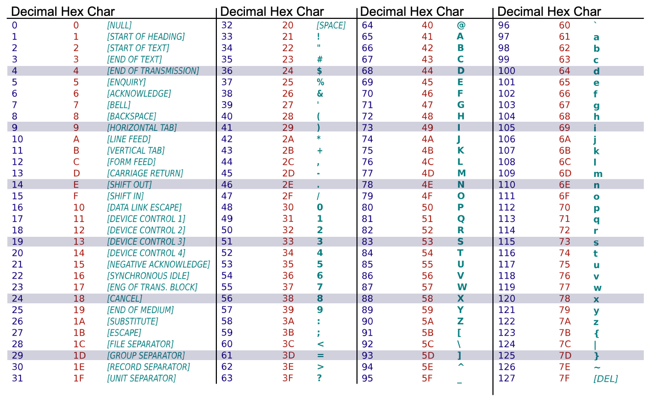
The ord built-in turns characters into their ASCII form.

Question

The largest value for a character is 127, can you guess why?

ASCII

American Standard Code for Information Interchange

Unicode is the new standard.

Random strings

The built-in chr function turns numbers into characters.

rnd.seed(1)
chars = [chr(rnd.randint(32, 127)) for _ in range(10)]
chars
['E', ',', 'h', ')', 'k', '%', 'o', '`', '0', '!']
" ".join(chars)
'E , h ) k % o ` 0 !'
"".join([chr(rnd.randint(32, 127)) for _ in range(50)])
"lg&9R42t+<=.Rdww~v-)'_]6Y! \\q(x-Oh>g#f5QY#d8Kl:TpI"
"".join([chr(rnd.randint(0, 128)) for _ in range(50)])
'R\x0f@D\x19obW\x07\x1a\x19h\x16\tCg~\x17}d\x1b%9S&\x08 "\n\x17\x0foW\x19Gs\\J>. X\x177AqM\x03\x00x'

Escape characters

print("Hello,\tworld!")
Hello,  world!
print("Line 1\nLine 2")
Line 1
Line 2
print("Patrick\rLaub")
Laubick
print("C:\tom\new folder")
C:  om
ew folder

Escape the backslash:

print("C:\\tom\\new folder")
C:\tom\new folder
repr("Hello,\rworld!")
"'Hello,\\rworld!'"

Non-natural language processing I

How would you evaluate

10 + 2 * -3

All that Python sees is a string of characters.

[ord(c) for c in "10 + 2 * -3"]
[49, 48, 32, 43, 32, 50, 32, 42, 32, 45, 51]
10 + 2 * -3
4

Non-natural language processing II

Python first tokenizes the string:

import tokenize
import io

code = "10 + 2 * -3"
tokens = tokenize.tokenize(io.BytesIO(code.encode("utf-8")).readline)
for token in tokens:
    print(token)
TokenInfo(type=63 (ENCODING), string='utf-8', start=(0, 0), end=(0, 0), line='')
TokenInfo(type=2 (NUMBER), string='10', start=(1, 0), end=(1, 2), line='10 + 2 * -3')
TokenInfo(type=54 (OP), string='+', start=(1, 3), end=(1, 4), line='10 + 2 * -3')
TokenInfo(type=2 (NUMBER), string='2', start=(1, 5), end=(1, 6), line='10 + 2 * -3')
TokenInfo(type=54 (OP), string='*', start=(1, 7), end=(1, 8), line='10 + 2 * -3')
TokenInfo(type=54 (OP), string='-', start=(1, 9), end=(1, 10), line='10 + 2 * -3')
TokenInfo(type=2 (NUMBER), string='3', start=(1, 10), end=(1, 11), line='10 + 2 * -3')
TokenInfo(type=4 (NEWLINE), string='', start=(1, 11), end=(1, 12), line='')
TokenInfo(type=0 (ENDMARKER), string='', start=(2, 0), end=(2, 0), line='')

Non-natural language processing III

Python needs to parse the tokens into an abstract syntax tree.

import ast

print(ast.dump(ast.parse("10 + 2 * -3"), indent="  "))
Module(
  body=[
    Expr(
      value=BinOp(
        left=Constant(value=10),
        op=Add(),
        right=BinOp(
          left=Constant(value=2),
          op=Mult(),
          right=UnaryOp(
            op=USub(),
            operand=Constant(value=3)))))],
  type_ignores=[])

graph TD;
    Expr --> C[Add]
    C --> D[10]
    C --> E[Mult]
    E --> F[2]
    E --> G[USub]
    G --> H[3]

Non-natural language processing IV

The abstract syntax tree is then compiled into bytecode.

import dis

def expression(a, b, c):
    return a + b * -c

dis.dis(expression)
  3           0 RESUME                   0

  4           2 LOAD_FAST                0 (a)
              4 LOAD_FAST                1 (b)
              6 LOAD_FAST                2 (c)
              8 UNARY_NEGATIVE
             10 BINARY_OP                5 (*)
             14 BINARY_OP                0 (+)
             18 RETURN_VALUE

Running the bytecode

Applications of NLP in Industry

1) Classifying documents: Using the language within a body of text to classify it into a particular category, e.g.:

  • Grouping emails into high and low urgency
  • Movie reviews into positive and negative sentiment (i.e. sentiment analysis)
  • Company news into bullish (positive) and bearish (negative) statements

2) Machine translation: Assisting language translators with machine-generated suggestions from a source language (e.g. English) to a target language

Applications of NLP in Industry

3) Search engine functions, including:

  • Autocomplete
  • Predicting what information or website user is seeking

4) Speech recognition: Interpreting voice commands to provide information or take action. Used in virtual assistants such as Alexa, Siri, and Cortana

Deep learning & NLP?

Simple NLP applications such as spell checkers and synonym suggesters do not require deep learning and can be solved with deterministic, rules-based code with a dictionary/thesaurus.

More complex NLP applications such as classifying documents, search engine word prediction, and chatbots are complex enough to be solved using deep learning methods.

NLP in 1966-1973 #1

A typical story occurred in early machine translation efforts, which were generously funded by the U.S. National Research Council in an attempt to speed up the translation of Russian scientific papers in the wake of the Sputnik launch in 1957. It was thought initially that simple syntactic transformations, based on the grammars of Russian and English, and word replacement from an electronic dictionary, would suffice to preserve the exact meanings of sentences.

NLP in 1966-1973 #2

The fact is that accurate translation requires background knowledge in order to resolve ambiguity and establish the content of the sentence. The famous retranslation of “the spirit is willing but the flesh is weak” as “the vodka is good but the meat is rotten” illustrates the difficulties encountered. In 1966, a report by an advisory committee found that “there has been no machine translation of general scientific text, and none is in immediate prospect.” All U.S. government funding for academic translation projects was canceled.

High-level history of deep learning

A brief history of deep learning.

Car Crash Police Reports

Downloading the dataset

Look at the (U.S.) National Highway Traffic Safety Administration’s (NHTSA) National Motor Vehicle Crash Causation Survey (NMVCCS) dataset.

1from pathlib import Path

2if not Path("NHTSA_NMVCCS_extract.parquet.gzip").exists():
    print("Downloading dataset")                                    
    !wget https://github.com/JSchelldorfer/ActuarialDataScience/raw/master/12%20-%20NLP%20Using%20Transformers/NHTSA_NMVCCS_extract.parquet.gzip
3
4df = pd.read_parquet("NHTSA_NMVCCS_extract.parquet.gzip")
5print(f"shape of DataFrame: {df.shape}")
1
Imports Path class from pathlib library
2
Checks whether the zip folder already exists
3
If it doesn’t, gets the folder from the given location
4
Reads the zipped parquet file and stores it as a data frame. parquet is an efficient data storage format, similar to .csv
5
Prints the shape of the data frame
shape of DataFrame: (6949, 16)

Features

  • level_0, index, SCASEID: all useless row numbers
  • SUMMARY_EN and SUMMARY_GE: summaries of the accident
  • NUMTOTV: total number of vehicles involved in the accident
  • WEATHER1 to WEATHER8:
    • WEATHER1: cloudy
    • WEATHER2: snow
    • WEATHER3: fog, smog, smoke
    • WEATHER4: rain
    • WEATHER5: sleet, hail (freezing drizzle or rain)
    • WEATHER6: blowing snow
    • WEATHER7: severe crosswinds
    • WEATHER8: other
  • INJSEVA and INJSEVB: injury severity & (binary) presence of bodily injury

The analysis will ignore variables level_0, index, SCASEID, SUMMARY_GE and INJSEVA.

Crash summaries

df["SUMMARY_EN"]
0       V1, a 2000 Pontiac Montana minivan, made a lef...
1       The crash occurred in the eastbound lane of a ...
2       This crash occurred just after the noon time h...
                              ...                        
6946    The crash occurred in the eastbound lanes of a...
6947    This single-vehicle crash occurred in a rural ...
6948    This two vehicle daytime collision occurred mi...
Name: SUMMARY_EN, Length: 6949, dtype: object

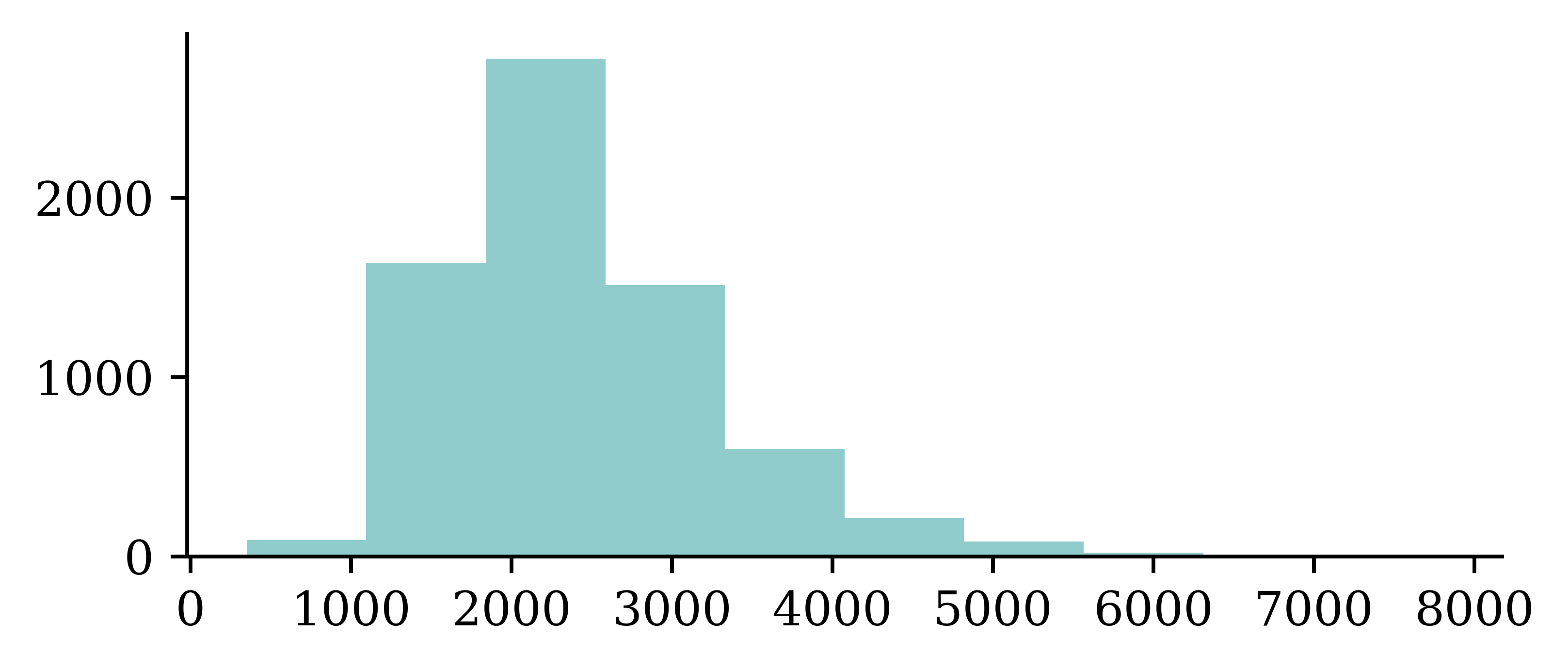
The SUMMARY_EN column contains summary of the accidents. There are 6949 rows corresponding to 6949 accidents. The data type is object, therefore, it will perform string (not mathematical) operations on the data. The following code shows how to generate a histogram for the length of the string. It looks at each entry of the column SUMMARY_EN, computes the length of the string (number of letters in the string), and create a histogram. The histogram shows that summaries are 2000 characters long on average.

df["SUMMARY_EN"].map(lambda summary: len(summary)).hist(grid=False);

A crash summary

The following code looks at the data entry for integer location 1 from the SUMMARY_EN data column in the dataframe df.

df["SUMMARY_EN"].iloc[1]
"The crash occurred in the eastbound lane of a two-lane, two-way asphalt roadway on level grade.  The conditions were daylight and wet with cloudy skies in the early afternoon on a weekday.\t\r \r V1, a 1995 Chevrolet Lumina was traveling eastbound.  V2, a 2004 Chevrolet Trailblazer was also traveling eastbound on the same roadway.  V2, was attempting to make a left-hand turn into a private drive on the North side of the roadway.  While turning V1 attempted to pass V2 on the left-hand side contacting it's front to the left side of V2.  Both vehicles came to final rest on the roadway at impact.\r \r The driver of V1 fled the scene and was not identified, so no further information could be obtained from him.  The Driver of V2 stated that the driver was a male and had hit his head and was bleeding.  She did not pursue the driver because she thought she saw a gun. The officer said that the car had been reported stolen.\r \r The Critical Precrash Event for the driver of V1 was this vehicle traveling over left lane line on the left side of travel.  The Critical Reason for the Critical Event was coded as unknown reason for the critical event because the driver was not available. \r \r The driver of V2 was a 41-year old female who had reported that she had stopped prior to turning to make sure she was at the right house.  She was going to show a house for a client.  She had no health related problems.  She had taken amoxicillin.  She does not wear corrective lenses and felt rested.  She was not injured in the crash.\r \r The Critical Precrash Event for the driver of V2 was other vehicle encroachment from adjacent lane over left lane line.  The Critical Reason for the Critical Event was not coded for this vehicle and the driver of V2 was not thought to have contributed to the crash."

Note that the output is with in double quotations. Further, we can see characters like \r \t in the output. This allows us to copy the entire output, and insert it in any python code for running codes. It is different from printing the output.

Carriage returns

print(df["SUMMARY_EN"].iloc[1])

Passing the print command for df["SUMMARY_EN"].iloc[1] returns an output without the double quotations. Furthermore, the characters like \r \t are now activated in to ‘carriage return’ and ‘tab’ controls respectively. If ‘carriage return’ characters are activated (without newline character \n following it), then it can write next text over the previous lines and create confusion in the text processing.

The Critical Precrash Event for the driver of V2 was other vehicle encroachment from adjacent lane over left lane line.  The Critical Reason for the Critical Event was not coded for this vehicle and the driver of V2 was not thought to have contributed to the crash.r corrective lenses and felt rested.  She was not injured in the crash. of V2.  Both vehicles came to final rest on the roadway at impact.

To avoid such confusions in text processing, we can write a function to replace \r character with \n in the following manner, and apply the function to the entire SUMMARY_EN column using the map function.

# Replace every \r with \n
def replace_carriage_return(summary):
    return summary.replace("\r", "\n")

df["SUMMARY_EN"] = df["SUMMARY_EN"].map(replace_carriage_return)
print(df["SUMMARY_EN"].iloc[1][:500])
The crash occurred in the eastbound lane of a two-lane, two-way asphalt roadway on level grade.  The conditions were daylight and wet with cloudy skies in the early afternoon on a weekday.    
 
 V1, a 1995 Chevrolet Lumina was traveling eastbound.  V2, a 2004 Chevrolet Trailblazer was also traveling eastbound on the same roadway.  V2, was attempting to make a left-hand turn into a private drive on the North side of the roadway.  While turning V1 attempted to pass V2 on the left-hand side contactin

Target

Predict number of vehicles in the crash.

df["NUMTOTV"].value_counts()\
1    .sort_index()
1
The code selects the column with total number of vehicles NUMTOTV, obtain the value counts for each categories, returns the sorted vector.
NUMTOTV
1    1822
2    4151
3     783
4     150
5      34
6       5
7       2
8       1
9       1
Name: count, dtype: int64
np.sum(df["NUMTOTV"] > 3)
193

Simplify the target to just:

  • 1 vehicle
  • 2 vehicles
  • 3+ vehicles
df["NUM_VEHICLES"] = \
  df["NUMTOTV"].map(lambda x: \
1    str(x) if x <= 2 else "3+")
df["NUM_VEHICLES"].value_counts()\
  .sort_index()
1
Writes a function to reduce categories to 3, by combining all categories with 3 or more vehicles into one category
NUM_VEHICLES
1     1822
2     4151
3+     976
Name: count, dtype: int64

Just ignore this for now…

rnd.seed(123)

for i, summary in enumerate(df["SUMMARY_EN"]):
    word_numbers = ["one", "two", "three", "four", "five", "six", "seven", "eight", "nine", "ten"]
    num_cars = 10
    new_car_nums = [f"V{rnd.randint(100, 10000)}" for _ in range(num_cars)]
    num_spaces = 4

    for car in range(1, num_cars+1):
        new_num = new_car_nums[car-1]
        summary = summary.replace(f"V-{car}", new_num)
        summary = summary.replace(f"Vehicle {word_numbers[car-1]}", new_num).replace(f"vehicle {word_numbers[car-1]}", new_num)
        summary = summary.replace(f"Vehicle #{word_numbers[car-1]}", new_num).replace(f"vehicle #{word_numbers[car-1]}", new_num)
        summary = summary.replace(f"Vehicle {car}", new_num).replace(f"vehicle {car}", new_num)
        summary = summary.replace(f"Vehicle #{car}", new_num).replace(f"vehicle #{car}", new_num)
        summary = summary.replace(f"Vehicle # {car}", new_num).replace(f"vehicle # {car}", new_num)

        for j in range(num_spaces+1):
            summary = summary.replace(f"V{' '*j}{car}", new_num).replace(f"V{' '*j}#{car}", new_num).replace(f"V{' '*j}# {car}", new_num)
            summary = summary.replace(f"v{' '*j}{car}", new_num).replace(f"v{' '*j}#{car}", new_num).replace(f"v{' '*j}# {car}", new_num)
         
    df.loc[i, "SUMMARY_EN"] = summary

Convert y to integers & split the data

1from sklearn.preprocessing import LabelEncoder
2target_labels = df["NUM_VEHICLES"]
3target = LabelEncoder().fit_transform(target_labels)
target
1
Imports the LabelEncoder from sklearn.preprocessing library
2
Defines the target variable
3
Fit and transform the target variable using LabelEncoder
array([1, 1, 1, ..., 2, 0, 1])
1weather_cols = [f"WEATHER{i}" for i in range(1, 9)]
2features = df[["SUMMARY_EN"] + weather_cols]

X_main, X_test, y_main, y_test = \
3    train_test_split(features, target, test_size=0.2, random_state=1)

# As 0.25 x 0.8 = 0.2
X_train, X_val, y_train, y_val = \
4    train_test_split(X_main, y_main, test_size=0.25, random_state=1)

5X_train.shape, X_val.shape, X_test.shape
1
Creates a list that returns column names of weather conditions, i.e. ['WEATHER1', 'WEATHER2', 'WEATHER3', 'WEATHER4', 'WEATHER5', 'WEATHER6', 'WEATHER7', 'WEATHER8']
2
Defines the feature vector by selecting relevant columns from the data frame df
3
Splits the data into train and validation sets
4
Further divides the validation set into validation set and test set
5
Prints the dimensions of the data frames
((4169, 9), (1390, 9), (1390, 9))
print([np.mean(y_train == y) for y in [0, 1, 2]])
[0.25833533221396016, 0.6032621731830176, 0.1384024946030223]

Text Vectorisation

Text vectorisation is a method to convert text into a numerical representation.

Grab the start of a few summaries

first_summaries = X_train["SUMMARY_EN"].iloc[:3]
first_summaries
2532    This crash occurred in the early afternoon of ...
6209    This two-vehicle crash occurred in a four-legg...
2561    The crash occurred in the eastbound direction ...
Name: SUMMARY_EN, dtype: object
1first_words = first_summaries.map(lambda txt: txt.split(" ")[:7])
first_words
1
Takes the first_summaries, converts the string of words in to a list of words by breaking the string at spaces and returns the first 7 words
2532    [This, crash, occurred, in, the, early, aftern...
6209    [This, two-vehicle, crash, occurred, in, a, fo...
2561    [The, crash, occurred, in, the, eastbound, dir...
Name: SUMMARY_EN, dtype: object
1start_of_summaries = first_words.map(lambda txt: " ".join(txt))
start_of_summaries
1
Joint the words in the list with a space in between to return a string
2532          This crash occurred in the early afternoon
6209    This two-vehicle crash occurred in a four-legged
2561       The crash occurred in the eastbound direction
Name: SUMMARY_EN, dtype: object

Count words in the first summaries

1from sklearn.feature_extraction.text import CountVectorizer

2vect = CountVectorizer()
3counts = vect.fit_transform(start_of_summaries)
4vocab = vect.get_feature_names_out()
print(len(vocab), vocab)
1
Imports the CountVectorizer class from the sklearn.feature_extraction.text library. CountVectorizer goes through a text document, identifies distinct words in it, and returns a sparse matrix.
2
Applies fit_transform function to the start_of_summaries
3
Stores the distinct words in the vector vocab
4
Returns the number of distinct words, and the words themselves
13 ['afternoon' 'crash' 'direction' 'early' 'eastbound' 'four' 'in' 'legged'
 'occurred' 'the' 'this' 'two' 'vehicle']
counts
<3x13 sparse matrix of type '<class 'numpy.int64'>'
    with 21 stored elements in Compressed Sparse Row format>

Giving the command to return counts does not return the matrix in full form. Since python saves the matrix in a Therefore, we use the following code.

counts.toarray()
array([[1, 1, 0, 1, 0, 0, 1, 0, 1, 1, 1, 0, 0],
       [0, 1, 0, 0, 0, 1, 1, 1, 1, 0, 1, 1, 1],
       [0, 1, 1, 0, 1, 0, 1, 0, 1, 2, 0, 0, 0]])

In the above matrix, rows correspond to the data entries (strings), columns correspond to distinct words, and cell entries correspond to the frequencies of distinct words in each row

Encode new sentences to BoW

vect.transform([
    "first car hit second car in a crash",
    "ipad os 16 beta released",
1])
1
Applies transform to two new lines of data. vect.transform applies the already fitted transformation to the new data. It goes through the new data entries, identifies words that were seen during fit_transform stage, and returns a matrix containing the counts of distinct words (identified during fitting stage).
<2x13 sparse matrix of type '<class 'numpy.int64'>'
    with 2 stored elements in Compressed Sparse Row format>

Note that the matrix is stored in a special format in python, hence, we must pass the command to convert it to an array using the following code.

vect.transform([
    "first car hit second car in a crash",
    "ipad os 16 beta released",
]).toarray()
array([[0, 1, 0, 0, 0, 0, 1, 0, 0, 0, 0, 0, 0],
       [0, 0, 0, 0, 0, 0, 0, 0, 0, 0, 0, 0, 0]])

There are couple issues with the output. Since the transform function, will identify only the words trained during the fit_transform stage, it will not recognize the new words. The returned matrix can only say whether new data contains words seen during the fitting stage or not. We can see how the matrix returns an entire row of zero values for the second line.

print(vocab)
['afternoon' 'crash' 'direction' 'early' 'eastbound' 'four' 'in' 'legged'
 'occurred' 'the' 'this' 'two' 'vehicle']

Bag of n-grams

The same CountVectorizer class can be customized to look at 2 words too. This is useful in some situations. For example, the word ‘new’ and ‘york’ separately might not be meaningful, but together, it can. This motivates the n-grams option. The following code CountVectorizer(ngram_range=(1, 2)) is an example of giving instructions to look for phrases with one word and two words.

vect = CountVectorizer(ngram_range=(1, 2))
counts = vect.fit_transform(start_of_summaries)
vocab = vect.get_feature_names_out()
print(len(vocab), vocab)
27 ['afternoon' 'crash' 'crash occurred' 'direction' 'early'
 'early afternoon' 'eastbound' 'eastbound direction' 'four' 'four legged'
 'in' 'in four' 'in the' 'legged' 'occurred' 'occurred in' 'the'
 'the crash' 'the early' 'the eastbound' 'this' 'this crash' 'this two'
 'two' 'two vehicle' 'vehicle' 'vehicle crash']
counts.toarray()
array([[1, 1, 1, 0, 1, 1, 0, 0, 0, 0, 1, 0, 1, 0, 1, 1, 1, 0, 1, 0, 1, 1,
        0, 0, 0, 0, 0],
       [0, 1, 1, 0, 0, 0, 0, 0, 1, 1, 1, 1, 0, 1, 1, 1, 0, 0, 0, 0, 1, 0,
        1, 1, 1, 1, 1],
       [0, 1, 1, 1, 0, 0, 1, 1, 0, 0, 1, 0, 1, 0, 1, 1, 2, 1, 0, 1, 0, 0,
        0, 0, 0, 0, 0]])

See: Google Books Ngram Viewer

TF-IDF

Stands for term frequency-inverse document frequency.

Infographic explaining TF-IDF

term frequency-inverse document frequency measures the importance of a word across documents. It first computes the frequency of term x in the document y and weights it by a measure of how common it is. The intuition here is that, the more the word x appears across documents, the less important it becomes.

Bag Of Words

Count words in all the summaries

1vect = CountVectorizer()
2vect.fit(X_train["SUMMARY_EN"])
3vocab = list(vect.get_feature_names_out())
4len(vocab)
1
Defines the class CountVectorizer() as vect
2
Fits the vectorizer to the entire column of SUMMARY_EN
3
Stores the distinct words as a list
4
Returns the number of unique words
18866

The above code returns 18866 number of unique words.

1vocab[:5], vocab[len(vocab)//2:(len(vocab)//2 + 5)], vocab[-5:]
1
Returns (i) the first five elements, (ii) the middle five elements and (iii) the last five elements of the array.
(['00', '000', '000lbs', '003', '005'],
 ['swinger', 'swinging', 'swipe', 'swiped', 'swiping'],
 ['zorcor', 'zotril', 'zx2', 'zx5', 'zyrtec'])

Create the X matrices

The following function is designed to select and vectorize the text column of a given dataset, and then combine it with the other non-textual columns of the same dataset.

1def vectorise_dataset(X, vect, txt_col="SUMMARY_EN", dataframe=False):
2    X_vects = vect.transform(X[txt_col]).toarray()
3    X_other = X.drop(txt_col, axis=1)

4    if not dataframe:
        return np.concatenate([X_vects, X_other], axis=1)                           
    else:
        # Add column names and indices to the combined dataframe.
5        vocab = list(vect.get_feature_names_out())
6        X_vects_df = pd.DataFrame(X_vects, columns=vocab, index=X.index)
7        return pd.concat([X_vects_df, X_other], axis=1)
1
Defines the function vectorise_dataset which takes in the dataframe X, vectorizer class, the name of the text column, a boolean function defining whether we want the output in dataframe format or numpy array format
2
Transforms the text column based on a already fitted vectorizer function
3
Drops the column containing text data from the dataframe
4
If dataframe=False, then returns a numpy array by concatenating non-textual data and vectorized text data
5
Otherwise, extracts the unique words as a list
6
Generates a dataframe, with columns names vocab, while preserving the index from the original dataset X
7
Concatenates X_vects_df with the remaining non-textual data and returns the output as a dataframe
X_train_ct = vectorise_dataset(X_train, vect)
X_val_ct = vectorise_dataset(X_val, vect)
X_test_ct = vectorise_dataset(X_test, vect)

Check the input matrix

vectorise_dataset(X_train, vect, dataframe=True)
00 000 000lbs 003 005 007 00am 00pm 00tydo2 01 ... zx5 zyrtec WEATHER1 WEATHER2 WEATHER3 WEATHER4 WEATHER5 WEATHER6 WEATHER7 WEATHER8
2532 0 0 0 0 0 0 0 0 0 0 ... 0 0 0 0 0 0 0 0 0 0
6209 0 0 0 0 0 0 0 0 0 0 ... 0 0 0 0 0 0 0 0 0 0
2561 0 0 0 0 0 0 0 0 0 0 ... 0 0 0 0 0 0 0 0 0 0
... ... ... ... ... ... ... ... ... ... ... ... ... ... ... ... ... ... ... ... ... ...
6882 0 0 0 0 0 0 0 0 0 0 ... 0 0 0 0 0 0 0 0 0 0
206 0 0 0 0 0 0 0 0 0 0 ... 0 0 0 0 0 0 0 0 0 0
6356 0 0 0 0 0 0 0 0 0 0 ... 0 0 0 0 0 0 0 0 0 0

4169 rows × 18874 columns

The above code returns the output matrix and it contains 4169 rows with 18874 columns. Next, we build a simple neural network on the data, to predict the probabilities of number of vehicles involved in the accident.

Make a simple dense model

1num_features = X_train_ct.shape[1]
2num_cats = 3 # 1, 2, 3+ vehicles

3def build_model(num_features, num_cats):
4    random.seed(42)
    
    model = Sequential([
        Input((num_features,)),
        Dense(100, activation="relu"),
        Dense(num_cats, activation="softmax")
5    ])
    
6    topk = SparseTopKCategoricalAccuracy(k=2, name="topk")
    model.compile("adam", "sparse_categorical_crossentropy",
7        metrics=["accuracy", topk])
    
    return model
1
Stores the number of input features in num_features
2
Stores the number of output features in num_cats
3
Starts building the model by giving number of input and output features as parameters
4
Sets the random seed for reproducibility
5
Constructs the neural network with 2 dense layers. Since the output must be a vector of probabilities, we choose softmax activation in the output layer
6
Defines the a customized metric to keep track of during the training. The metric will compute the accuracy by looking at top 2 classes(the 2 classes with highest predicted probability) and checking if either of them contains the true class
7
Compiles the model with the adam optimizer, loss function and metrics to monitor. Here we ask the model to optimize sparse_categorical_crossentropy loss while keeping track of sparse_categorical_crossentropy for the top 2 classes ## Inspect the model
model = build_model(num_features, num_cats)
model.summary()
Model: "sequential"
┏━━━━━━━━━━━━━━━━━━━━━━━━━━━━━━━━━┳━━━━━━━━━━━━━━━━━━━━━━━━┳━━━━━━━━━━━━━━━┓
┃ Layer (type)                     Output Shape                  Param # ┃
┡━━━━━━━━━━━━━━━━━━━━━━━━━━━━━━━━━╇━━━━━━━━━━━━━━━━━━━━━━━━╇━━━━━━━━━━━━━━━┩
│ dense (Dense)                   │ (None, 100)            │     1,887,500 │
├─────────────────────────────────┼────────────────────────┼───────────────┤
│ dense_1 (Dense)                 │ (None, 3)              │           303 │
└─────────────────────────────────┴────────────────────────┴───────────────┘
 Total params: 1,887,803 (7.20 MB)
 Trainable params: 1,887,803 (7.20 MB)
 Non-trainable params: 0 (0.00 B)

The model summary shows that there are 1,887,803 parameters to learn. This is because we have 188500 (18874*100 weights + 100 biases) parameters to train in the first layer.

Fit & evaluate the model

es = EarlyStopping(patience=1, restore_best_weights=True,
    monitor="val_accuracy", verbose=2)
%time hist = model.fit(X_train_ct, y_train, epochs=10, \
    callbacks=[es], validation_data=(X_val_ct, y_val), verbose=0);
Epoch 3: early stopping
Restoring model weights from the end of the best epoch: 2.
CPU times: user 2.51 s, sys: 1.65 s, total: 4.17 s
Wall time: 4.2 s

Results from training the neural network shows that the model performs almost perfectly for the in sample data, and with very high accuracies for both validation and test data.

model.evaluate(X_train_ct, y_train, verbose=0)
[0.015506910160183907, 1.0, 1.0]
model.evaluate(X_val_ct, y_val, verbose=0)
[0.16680333018302917, 0.9525179862976074, 0.9956834316253662]
model.evaluate(X_test_ct, y_test, verbose=0)
[0.17666228115558624, 0.9417266249656677, 0.9978417158126831]

Limiting The Vocabulary

Although the previous model performed really well, it had a very large number of parameters to train. Therefore, it is worth checking whether there is a way to limit the vocabulary. One way would be to look at only the most frequent words occurring

The max_features value

One way would be to select the most frequent words. The following code shows how we can choose max_features option to select the 10 words that occur most. This simplifies the problem, however, we might miss out on important words that might add value to the task. For example, and, for and of are among the selected words, but they are less meaningful.

vect = CountVectorizer(max_features=10)
vect.fit(X_train["SUMMARY_EN"])
vocab = vect.get_feature_names_out()
len(vocab)
10
print(vocab)
['and' 'driver' 'for' 'in' 'lane' 'of' 'the' 'to' 'vehicle' 'was']

Remove stop words

One way to overcome selecting less meaningful words would be to use the option 'stop_words="english' option. This option checks if the set of selected words contain common words, and ignore them when selecting the most frequent words.

vect = CountVectorizer(max_features=10, stop_words="english")
vect.fit(X_train["SUMMARY_EN"])
vocab = vect.get_feature_names_out()
len(vocab)
10
print(vocab)
['coded' 'crash' 'critical' 'driver' 'event' 'intersection' 'lane' 'left'
 'roadway' 'vehicle']

Keep 1,000 most frequent words

vect = CountVectorizer(max_features=1_000, stop_words="english")
vect.fit(X_train["SUMMARY_EN"])
vocab = vect.get_feature_names_out()
len(vocab)
1000
print(vocab[:5], vocab[len(vocab)//2:(len(vocab)//2 + 5)], vocab[-5:])
['10' '105' '113' '12' '15'] ['interruption' 'intersected' 'intersecting' 'intersection' 'interstate'] ['year' 'years' 'yellow' 'yield' 'zone']

The above output shows, how selecting just 1000 words would still contain less meaningful phrases. Also, we can see how the same word(but slightly differently spelled) are appearing together. This redundancy does not add value either. For example year and years.

Create the X matrices:

X_train_ct = vectorise_dataset(X_train, vect)
X_val_ct = vectorise_dataset(X_val, vect)
X_test_ct = vectorise_dataset(X_test, vect)

Check the input matrix

vectorise_dataset(X_train, vect, dataframe=True)
10 105 113 12 15 150 16 17 18 180 ... yield zone WEATHER1 WEATHER2 WEATHER3 WEATHER4 WEATHER5 WEATHER6 WEATHER7 WEATHER8
2532 0 0 0 0 0 0 0 0 0 0 ... 0 0 0 0 0 0 0 0 0 0
6209 0 0 0 0 0 0 0 0 0 0 ... 0 0 0 0 0 0 0 0 0 0
2561 1 0 1 0 0 0 0 0 0 0 ... 0 0 0 0 0 0 0 0 0 0
... ... ... ... ... ... ... ... ... ... ... ... ... ... ... ... ... ... ... ... ... ...
6882 0 0 0 0 0 0 0 0 0 0 ... 0 0 0 0 0 0 0 0 0 0
206 0 0 0 0 0 0 0 0 0 0 ... 0 0 0 0 0 0 0 0 0 0
6356 0 0 0 0 0 0 0 0 0 0 ... 0 0 0 0 0 0 0 0 0 0

4169 rows × 1008 columns

Make & inspect the model

num_features = X_train_ct.shape[1]
model = build_model(num_features, num_cats)
model.summary()
Model: "sequential_1"
┏━━━━━━━━━━━━━━━━━━━━━━━━━━━━━━━━━┳━━━━━━━━━━━━━━━━━━━━━━━━┳━━━━━━━━━━━━━━━┓
┃ Layer (type)                     Output Shape                  Param # ┃
┡━━━━━━━━━━━━━━━━━━━━━━━━━━━━━━━━━╇━━━━━━━━━━━━━━━━━━━━━━━━╇━━━━━━━━━━━━━━━┩
│ dense_2 (Dense)                 │ (None, 100)            │       100,900 │
├─────────────────────────────────┼────────────────────────┼───────────────┤
│ dense_3 (Dense)                 │ (None, 3)              │           303 │
└─────────────────────────────────┴────────────────────────┴───────────────┘
 Total params: 101,203 (395.32 KB)
 Trainable params: 101,203 (395.32 KB)
 Non-trainable params: 0 (0.00 B)

From the above summary, we can see how we have brought down the number of parameters to be trained down to 101,203. That is done by reducing the number of covariates, not by reducing the number of neurons.

Fit & evaluate the model

es = EarlyStopping(patience=1, restore_best_weights=True,
    monitor="val_accuracy", verbose=2)
%time hist = model.fit(X_train_ct, y_train, epochs=10, \
    callbacks=[es], validation_data=(X_val_ct, y_val), verbose=0);
Epoch 2: early stopping
Restoring model weights from the end of the best epoch: 1.
CPU times: user 352 ms, sys: 18.6 ms, total: 370 ms
Wall time: 373 ms

The following results show how despite dropping so many covariates, the trained model is still able to achieve a performance similar to the previous case.

model.evaluate(X_train_ct, y_train, verbose=0)
[0.1614694595336914, 0.9573038816452026, 0.9988006949424744]
model.evaluate(X_val_ct, y_val, verbose=0)
[0.22757881879806519, 0.9258992671966553, 0.9942445755004883]

Intelligently Limit The Vocabulary

While it is helpful to reduce complexity and redundancy in natural language processing using options like max_features and stop_words, they alone are not enough. The following code shows how despite using above commands, we still end up with similar words which do not add value for the processing task. Therefore, looking for ways to intelligently limit vocabulary is useful.

Keep 1,000 most frequent words

vect = CountVectorizer(max_features=1_000, stop_words="english")
vect.fit(X_train["SUMMARY_EN"])
vocab = vect.get_feature_names_out()
len(vocab)
1000
print(vocab[:5], vocab[len(vocab)//2:(len(vocab)//2 + 5)], vocab[-5:])
['10' '105' '113' '12' '15'] ['interruption' 'intersected' 'intersecting' 'intersection' 'interstate'] ['year' 'years' 'yellow' 'yield' 'zone']

Spacy is a popular open-source library that is used to analyse data and carry out prediction tasks related to natural language processing.

Install spacy

1!pip install spacy
2!python -m spacy download en_core_web_sm
1
Installs the library spacy
2
Downloads the trained model en_core_web_sm which a small, efficient English language model trained using text data. It can be used for tasks like lemmatization, tokenization etc.
1import spacy

2nlp = spacy.load("en_core_web_sm")
3doc = nlp("Apple is looking at buying U.K. startup for $1 billion")
for token in doc:
4    print(token.text, token.pos_, token.dep_)
1
Imports the library
2
Loads the model and stores it as nlp
3
Applies nlp model to the given string for processing. Processing involves tokenization, part-of-speech application, dependency application etc.
4
Returns information about each token(word) in the line. token.text returns each word in the string, token.pos_ returns the part-of-speech; the grammatical category of the word, and token.dep_ which provides information about the syntactic relationship of the word to the rest of the words in the string.
Apple PROPN nsubj
is AUX aux
looking VERB ROOT
at ADP prep
buying VERB pcomp
U.K. PROPN dobj
startup NOUN dobj
for ADP prep
$ SYM quantmod
1 NUM compound
billion NUM pobj

Lemmatize the text

Lemmatization refers to the act of reducing the words in to its base form. For example; reduced form of looking would be look. The following code shows how we can lemmatize the a text, by first processing it with nlp.

1def lemmatize(txt):
2    doc = nlp(txt)
    good_tokens = [token.lemma_.lower() for token in doc \
        if not token.like_num and \
           not token.is_punct and \
           not token.is_space and \
           not token.is_currency and \
3           not token.is_stop]
4    return " ".join(good_tokens)
1
Starts defining the function which taken in a string of text as input
2
Sends the text through nlp model
3
For each token(word) in the document, first it takes the lemma of the token, converts it to lower case and then applies several filters on the lemmatized token to select only the good tokens. The filtering process filters out numbers, punctuation marks, white spaces, currency signs and stop words like the and and
4
Joins the good tokens and returns it as a string
test_str = "Incident at 100kph and '10 incidents -13.3%' are incidental?\t $5"
lemmatize(test_str)
'incident 100kph incident incidental'
test_str = "I interviewed 5-years ago, 150 interviews every year at 10:30 are.."
lemmatize(test_str)
'interview year ago interview year 10:30'

The output above shows how stop words, numbers and punctuation marks are removed. We can also see how incident and incidental are treated as separate words.

Lemmatizing data in the above manner, giving each string at a time is quite inefficient. We can use map(lemmatize) function to map the function to the entire column at once.

Apply to the whole dataset

df["SUMMARY_EN_LEMMA"] = df["SUMMARY_EN"].map(lemmatize)

Lemmatized version of the column is now stored in SUMMARY_EN_LEMM. Next we merge the non-textual columns of the dataset df with the lemmatized column and create the final dataset. This dataset will be split in to train, val and test sets for training the neural network.

1weather_cols = [f"WEATHER{i}" for i in range(1, 9)]
2features = df[["SUMMARY_EN_LEMMA"] + weather_cols]

X_main, X_test, y_main, y_test = \
3    train_test_split(features, target, test_size=0.2, random_state=1)

# As 0.25 x 0.8 = 0.2
X_train, X_val, y_train, y_val = \
4    train_test_split(X_main, y_main, test_size=0.25, random_state=1)

5X_train.shape, X_val.shape, X_test.shape
1
Defines the names of the columns that will be used for creating the final dataset
2
Selects the relevant input feature columns and stores it in features column
3
Splits the data in to main and test sets
4
Further splits the main set in to train and val sets
5
Returns the dimensions of the datasets
((4169, 9), (1390, 9), (1390, 9))

Keep 1,000 most frequent lemmas

vect = CountVectorizer(max_features=1_000, stop_words="english")
vect.fit(X_train["SUMMARY_EN_LEMMA"])
vocab = vect.get_feature_names_out()
len(vocab)
1000

The output after lemmatization, when compared with the previous output (with 1000 words) does not contain similar words.

print(vocab[:5], vocab[len(vocab)//2:(len(vocab)//2 + 5)], vocab[-5:])
['10' '150' '48kmph' '4x4' '56kmph'] ['let' 'level' 'lexus' 'license' 'light'] ['yaw' 'year' 'yellow' 'yield' 'zone']

The following code demonstrates the steps for training a neural network using lemmatized datasets:

  1. We start by using the vectorise_dataset function to convert the text data into numerical vectors.
  2. Next, we train the neural network model using the vectorized dataset.
  3. Finally, we assess the model’s performance

Create the X matrices:

X_train_ct = vectorise_dataset(X_train, vect, "SUMMARY_EN_LEMMA")
X_val_ct = vectorise_dataset(X_val, vect, "SUMMARY_EN_LEMMA")
X_test_ct = vectorise_dataset(X_test, vect, "SUMMARY_EN_LEMMA")

Check the input matrix

vectorise_dataset(X_train, vect, "SUMMARY_EN_LEMMA", dataframe=True)
10 150 48kmph 4x4 56kmph 64kmph 72kmph ability able accelerate ... yield zone WEATHER1 WEATHER2 WEATHER3 WEATHER4 WEATHER5 WEATHER6 WEATHER7 WEATHER8
2532 0 0 0 0 0 0 0 0 0 0 ... 0 0 0 0 0 0 0 0 0 0
6209 0 0 0 0 0 0 0 0 0 0 ... 0 0 0 0 0 0 0 0 0 0
2561 0 0 0 0 1 1 0 0 0 0 ... 0 0 0 0 0 0 0 0 0 0
... ... ... ... ... ... ... ... ... ... ... ... ... ... ... ... ... ... ... ... ... ...
6882 0 0 0 0 0 0 0 0 0 0 ... 0 0 0 0 0 0 0 0 0 0
206 0 0 0 0 0 0 0 0 0 0 ... 0 0 0 0 0 0 0 0 0 0
6356 0 0 0 0 0 0 0 0 0 0 ... 0 0 0 0 0 0 0 0 0 0

4169 rows × 1008 columns

Make & inspect the model

num_features = X_train_ct.shape[1]
model = build_model(num_features, num_cats)
model.summary()
Model: "sequential_2"
┏━━━━━━━━━━━━━━━━━━━━━━━━━━━━━━━━━┳━━━━━━━━━━━━━━━━━━━━━━━━┳━━━━━━━━━━━━━━━┓
┃ Layer (type)                     Output Shape                  Param # ┃
┡━━━━━━━━━━━━━━━━━━━━━━━━━━━━━━━━━╇━━━━━━━━━━━━━━━━━━━━━━━━╇━━━━━━━━━━━━━━━┩
│ dense_4 (Dense)                 │ (None, 100)            │       100,900 │
├─────────────────────────────────┼────────────────────────┼───────────────┤
│ dense_5 (Dense)                 │ (None, 3)              │           303 │
└─────────────────────────────────┴────────────────────────┴───────────────┘
 Total params: 101,203 (395.32 KB)
 Trainable params: 101,203 (395.32 KB)
 Non-trainable params: 0 (0.00 B)

Fit & evaluate the model

es = EarlyStopping(patience=1, restore_best_weights=True,
    monitor="val_accuracy", verbose=2)
%time hist = model.fit(X_train_ct, y_train, epochs=10, \
    callbacks=[es], validation_data=(X_val_ct, y_val), verbose=0);
Epoch 2: early stopping
Restoring model weights from the end of the best epoch: 1.
CPU times: user 354 ms, sys: 1.84 ms, total: 356 ms
Wall time: 357 ms
model.evaluate(X_train_ct, y_train, verbose=0)
[0.1701967567205429, 0.9573038816452026, 0.9988006949424744]
model.evaluate(X_val_ct, y_val, verbose=0)
[0.25785908102989197, 0.9136690497398376, 0.9942445755004883]

Interrogate The Model

Trained neural networks performing really well on predictions does not necessarily imply good performance. Interrogating the model can help us understand inside workings of the model to ensure there are no underlying problems with model.

Permutation importance algorithm

Taken directly from scikit-learn documentation:

  • Inputs: fitted predictive model m, tabular dataset (training or validation) D.

  • Compute the reference score s of the model m on data D (for instance the accuracy for a classifier or the R^2 for a regressor).

  • For each feature j (column of D):

    • For each repetition k in {1, \dots, K}:

      • Randomly shuffle column j of dataset D to generate a corrupted version of the data named \tilde{D}_{k,j}.
      • Compute the score s_{k,j} of model m on corrupted data \tilde{D}_{k,j}.
    • Compute importance i_j for feature f_j defined as:

      i_j = s - \frac{1}{K} \sum_{k=1}^{K} s_{k,j}

Find important inputs

def permutation_test(model, X, y, num_reps=1, seed=42):
    """
    Run the permutation test for variable importance.
    Returns matrix of shape (X.shape[1], len(model.evaluate(X, y))).
    """
    rnd.seed(seed)
    scores = []    

    for j in range(X.shape[1]):
        original_column = np.copy(X[:, j])
        col_scores = []

        for r in range(num_reps):
            rnd.shuffle(X[:,j])
            col_scores.append(model.evaluate(X, y, verbose=0))

        scores.append(np.mean(col_scores, axis=0))
        X[:,j] = original_column
    
    return np.array(scores)

Run the permutation test

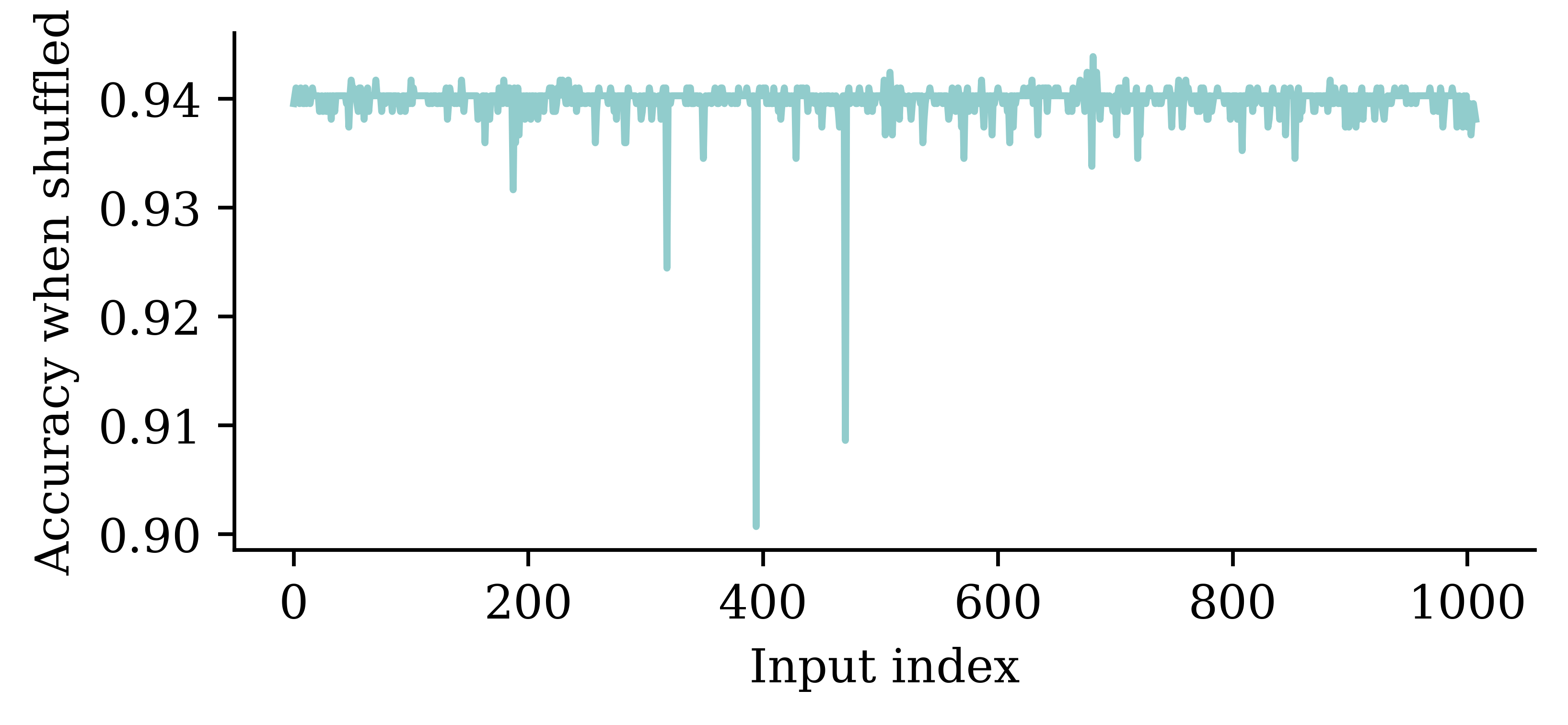
1perm_scores = permutation_test(model, X_val_ct, y_val)[:,1]
2plt.plot(perm_scores);
3plt.xlabel("Input index"); plt.ylabel("Accuracy when shuffled");
1
The permutation_test, aims to evaluate the model’s performance on different sets of unseen data. The idea here is to shuffle the order of the val set, and compare the model performance. [:,1] part will extract the accuracy of the output from the model evaluation and store is as a vector.
2
Plots the permutation scores
3
Labels x and y axes

The above method on a high-level says that, if we corrupt the information contained in a feature by changing the order of the data in that feature column, then we are able to see how much information the variable brings in. If a certain variable is not contributing to the prediction accuracy, then changing the order of the variable will not result in a notable drop in accuracy. However, if a certain variable is highly important, then changing the order of data will result in a larger drop. This is an indication of variable importance. The plot above shows how model’s accuracy fluctuates across variables, and we can see how certain variables result in larger drops of accuracies.

Find the most significant inputs

1vocab = vect.get_feature_names_out()
2input_cols = list(vocab) + weather_cols

3best_input_inds = np.argsort(perm_scores)[:100]
4best_inputs = [input_cols[idx] for idx in best_input_inds]

5print(best_inputs)
1
Extracts the names of the features in a vectorizer object
2
Combines the list of names in the vectorizer object with the weather columns
3
Sorts the perm_scores in the ascending order and select the 100 observation which had the most impact on model’s accuracy
4
Find the names of the input features by mapping the index
5
Prints the output
['harmful', 'involve', 'event', 'lane', 'rear', 'code', 'single', 'year', 'park', 'edge', 'traffic', 'medication', 'north', 'dry', 'cross', 'impact', 'asphalt', 'male', 'barrier', 'motor', 'intersection', 'critical', 'tree', 'try', 'drive', 'turn', 'afternoon', 'direction', 'familiar', 'female', 'pickup', 'line', 'WEATHER4', 'light', 'WEATHER2', 'reason', 'assign', 'undivided', 'look', 'car', 'southbound', 'legally', 'control', 'kmph', 'occur', 'overcompensation', 'curb', 'rush', 'strike', 'quarter', 'WEATHER8', 'weekday', 'WEATHER5', 'complete', 'counterclockwise', 'forward', 'street', 'recognition', 'transport', 'bind', 'driver', 'kph', 'wall', 'old', 'bmw', 'action', 'change', 'pedestrian', 'distraction', 'grassy', 'sideswipe', 'directional', 'ground', 'shoulder', 'past', 'help', 'route', 'decelerate', 'hear', 'stop', 'realize', 'weekly', 'encroachment', 'contact', 'pre', 'WEATHER7', 'ford', 'lexus', 'continue', 'lot', 'push', 'exist', 'contribute', 'cloudy', 'close', 'force', 'failure', 'poor', 'shopping', 'northeast']

How about a simple decision tree?

We can try building a simpler model using only the most important features. Here, we chose a classification decision tree.

1from sklearn import tree
2clf = tree.DecisionTreeClassifier(random_state=0, max_leaf_nodes=3)
3clf.fit(X_train_ct[:, best_input_inds], y_train);
1
Imports tree class from sklearn
2
Specifies a decision tree with 3 leaf nodes. max_leaf_nodes=3 ensures that the fitted tree will have at most 3 leaf nodes
3
Fits the decision tree on the selected dataset. Here we only select the best_input_inds columns from the train set
print(clf.score(X_train_ct[:, best_input_inds], y_train))
print(clf.score(X_val_ct[:, best_input_inds], y_val))
0.920844327176781
0.9330935251798561

The decision tree ends up giving pretty good results.

Decision tree

tree.plot_tree(clf, feature_names=best_inputs, filled=True);

print(np.where(clf.feature_importances_ > 0)[0])
[best_inputs[ind] for ind in np.where(clf.feature_importances_ > 0)[0]]
[ 0 35]
['harmful', 'reason']

Using the original dataset

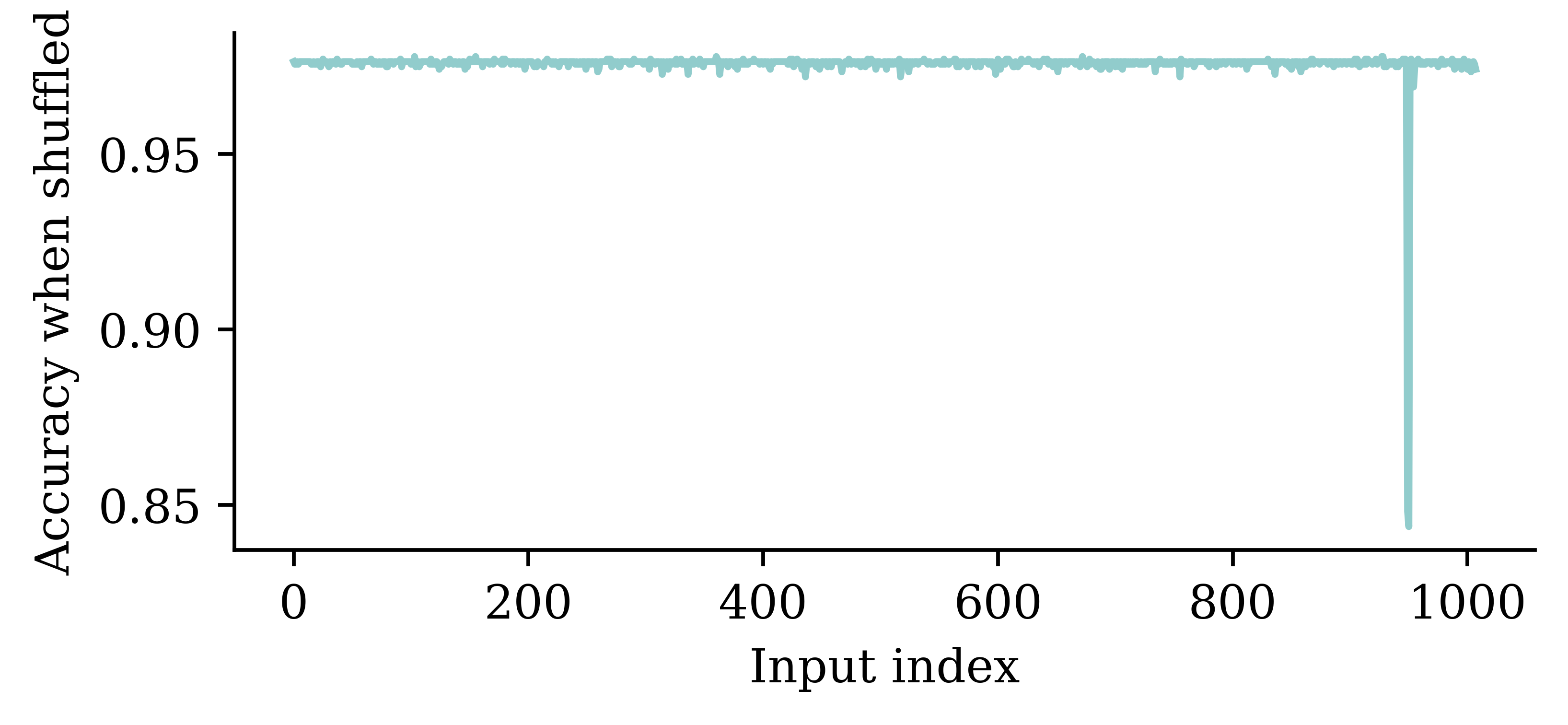
perm_scores = permutation_test(model, X_val_ct, y_val)[:,1]
plt.plot(perm_scores);
plt.xlabel("Input index"); plt.ylabel("Accuracy when shuffled");

Find the most significant inputs

vocab = vect.get_feature_names_out()
input_cols = list(vocab) + weather_cols

best_input_inds = np.argsort(perm_scores)[:100]
best_inputs = [input_cols[idx] for idx in best_input_inds]

print(best_inputs)
['v3', 'v2', 'involved', 'road', 'coded', 'impact', 'harmful', 'parked', 'WEATHER3', 'event', 'edge', 'v4', 'single', 'year', 'bituminous', 'WEATHER8', 'conditions', 'pushed', 'legally', 'came', 'vehicle', 'line', 'WEATHER5', 'WEATHER4', 'crash', 'WEATHER1', 'towed', 'cm', 'downhill', 'generally', 'highway', 'slope', 'higher', 'straight', 'brake', 'stopped', 'direction', 'occurred', 'critical', 'turning', 'WEATHER7', 'looked', 'way', 'trailer', 'let', 'driven', 'wet', 'precrash', 'location', 'went', 'light', 'continued', 'sign', 'motor', 'controlled', 'barrier', '30', 'illegal', 'events', 'steer', 'police', 'exit', 'steering', 'curve', 'daily', 'damage', 'failed', 'headed', 'route', 'northbound', 'poor', 'blazer', 'avoid', 'near', 'facing', 'posted', 'belted', 'cadillac', 'non', '1998', 'nissan', 'began', 'suffered', 'hearing', 'curb', 'right', 'picked', 'sedan', 'outside', 'fast', 'conversation', 'skidded', 'free', 'ford', 'setting', 'comprised', 'seven', 'condition', 'flow', 'passengers']

How about a simple decision tree?

clf = tree.DecisionTreeClassifier(random_state=0, max_leaf_nodes=3)
clf.fit(X_train_ct[:, best_input_inds], y_train);
print(clf.score(X_train_ct[:, best_input_inds], y_train))
print(clf.score(X_val_ct[:, best_input_inds], y_val))
0.9275605660829935
0.939568345323741

Decision tree

tree.plot_tree(clf, feature_names=best_inputs, filled=True);

The tree shows how, the model would check for the word v3, and decides the prediction as 3+. This is not very meaningful, because having v3 in the input is a direct indication of the number of vehicles.

print(np.where(clf.feature_importances_ > 0)[0])
[best_inputs[ind] for ind in np.where(clf.feature_importances_ > 0)[0]]
[ 0 38]
['v3', 'critical']

Word Embeddings

Overview

In order for deep learning models to process language, we need to supply that language to the model in a way it can digest, i.e. a quantitative representation such as a 2-D matrix of numerical values.

Popular methods for converting text into numbers include:

  • One-hot encoding
  • Bag of words
  • TF-IDF
  • Word vectors (transfer learning)

Assigning Numbers

Word Vectors

  • One-hot representations capture word ‘existence’ only, whereas word vectors capture information about word meaning as well as location.
  • This enables deep learning NLP models to automatically learn linguistic features.
  • Word2Vec & GloVe are popular algorithms for generating word embeddings (i.e. word vectors).

Word Vectors

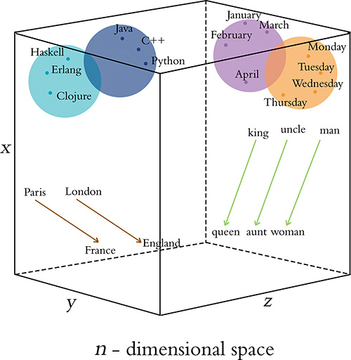
Illustrative word vectors.

Word vectors are a type of word embedding which can return numerical representations of words in a continuous vector space. There representations capture semantic knowledge of the words. For example, we can see how days are positioned closer to each other in a n-dimensional space.

  • Overarching concept is to assign each word within a corpus to a particular, meaningful location within a multidimensional space called the vector space.
  • Initially each word is assigned to a random location.
  • BUT by considering the words that tend to be used around a given word within the corpus, the locations of the words shift.

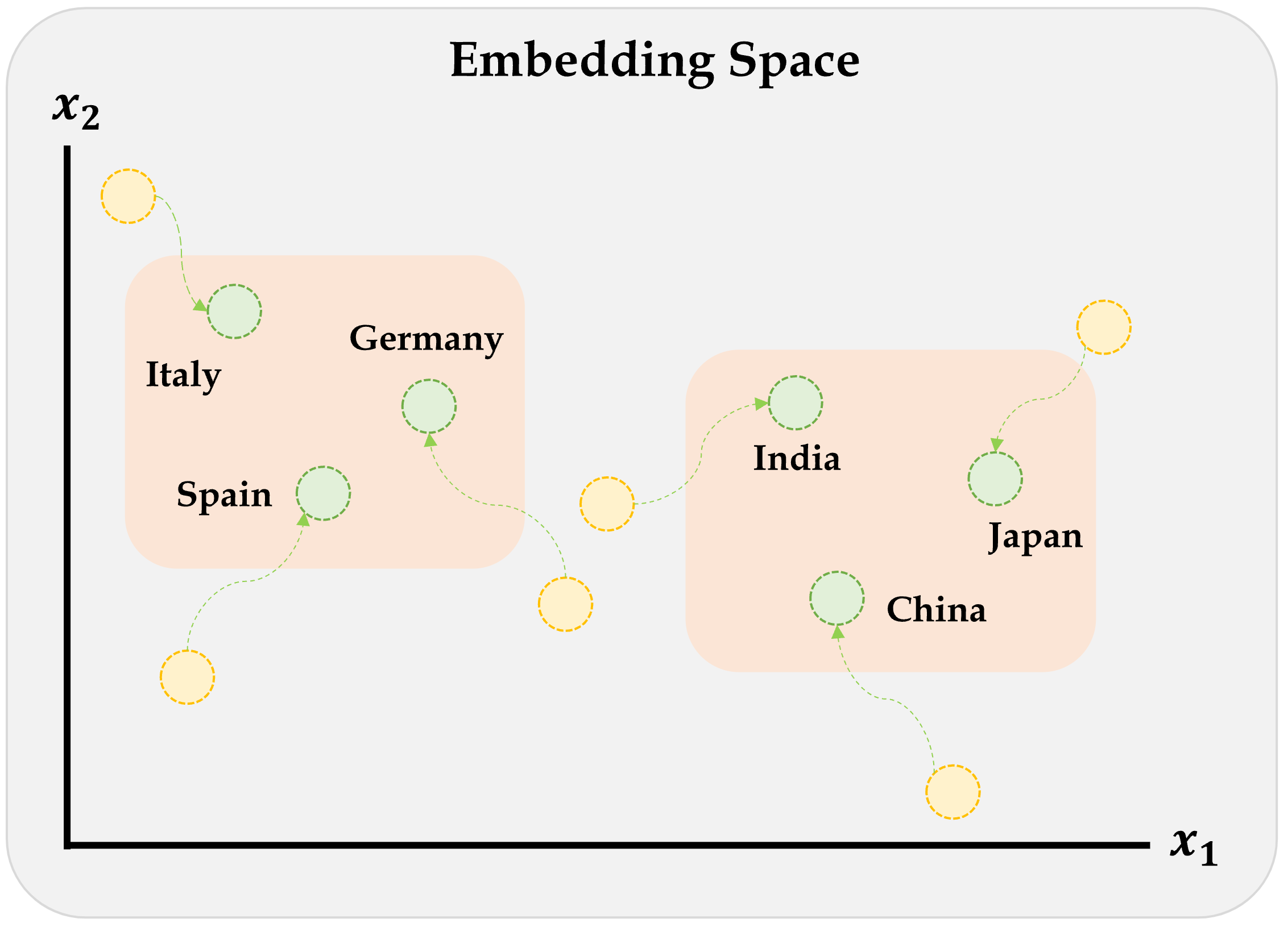
Remember this diagram?

Embeddings will gradually improve during training.

Embeddings are numerical representations of categorical data that were learned during the supervised learning process. However, numerical representations like Word2Vec & GloVe are popular algorithms for generating word embeddings that were trained by others, i.e. they are pretrained.

Word2Vec

Key idea: You’re known by the company you keep.

Two algorithms are used to calculate embeddings:

  • Continuous bag of words: uses the context words to predict the target word
  • Skip-gram: uses the target word to predict the context words

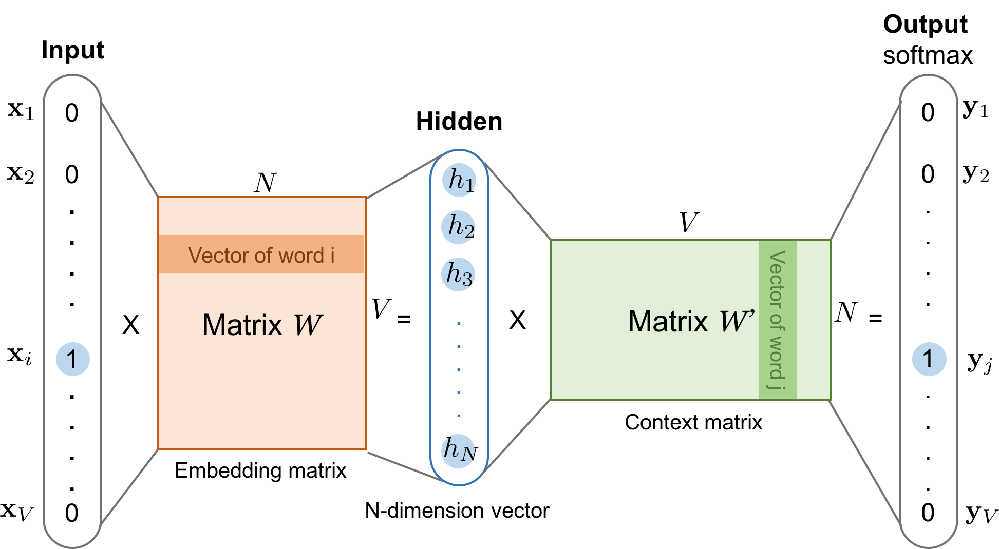
Predictions are made using a neural network with one hidden layer. Through backpropagation, we update a set of “weights” which become the word vectors.

Word2Vec training methods

Continuous bag of words is a center word prediction task

Skip-gram is a neighbour word prediction task
Suggested viewing

Computerphile (2019), Vectoring Words (Word Embeddings), YouTube (16 mins).

The skip-gram network

The skip-gram model. Both the input vector \boldsymbol{x} and the output \boldsymbol{y} are one-hot encoded word representations. The hidden layer is the word embedding of size N.

Word Vector Arithmetic

Relationships between words becomes vector math.

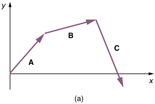
You remember vectors, right?
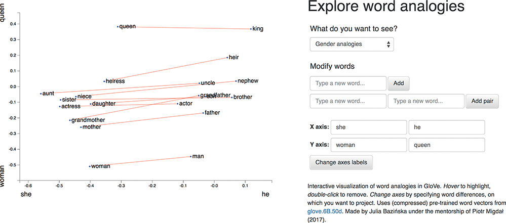
  • E.g., if we calculate the direction and distance between the coordinates of the words Paris and France, and trace this direction and distance from London, we should be close to the word England.

Illustrative word vector arithmetic

Screenshot from Word2viz

Word Embeddings II

Pretrained word embeddings

1!pip install gensim
1
Imports the gensim library. This is a popular library for document analysis

Load word2vec embeddings trained on Google News:

1import gensim.downloader as api
2wv = api.load('word2vec-google-news-300')
1
Imports the gensim.downloader module from the gensim library and stores is as api. This module contains pretrained models including Word2Vec and GloVe that can be used for NLP tasks
2
Loads the Word2Vec from the word2vec-google-news-300 dataset and stores is as wv

When run for the first time, that downloads a huge file:

gensim_dir = Path("~/gensim-data/").expanduser()
[str(p) for p in gensim_dir.iterdir()]
['/Users/plaub/gensim-data/.DS_Store',
 '/Users/plaub/gensim-data/word2vec-google-news-300',
 '/Users/plaub/gensim-data/information.json']
next(gensim_dir.glob("*/*.gz")).stat().st_size / 1024**3
1.6238203644752502
f"The size of the vocabulary is {len(wv)}"
'The size of the vocabulary is 3000000'

Treat wv like a dictionary

wv["pizza"]
array([-1.26e-01,  2.54e-02,  1.67e-01,  5.51e-01, -7.67e-02,  1.29e-01,
        1.03e-01, -3.95e-04,  1.22e-01,  4.32e-02,  1.73e-01, -6.84e-02,
        3.42e-01,  8.40e-02,  6.69e-02,  2.68e-01, -3.71e-02, -5.57e-02,
        1.81e-01,  1.90e-02, -5.08e-02,  9.03e-03,  1.77e-01,  6.49e-02,
       -6.25e-02, -9.42e-02, -9.72e-02,  4.00e-01,  1.15e-01,  1.03e-01,
       -1.87e-02, -2.70e-01,  1.81e-01,  1.25e-01, -3.17e-02, -5.49e-02,
        3.46e-01, -1.57e-02,  1.82e-05,  2.07e-01, -1.26e-01, -2.83e-01,
        2.00e-01,  8.35e-02, -4.74e-02, -3.11e-02, -2.62e-01,  1.70e-01,
       -2.03e-02,  1.53e-01, -1.21e-01,  3.75e-01, -5.69e-02, -4.76e-03,
       -1.95e-01, -2.03e-01,  3.01e-01, -1.01e-01, -3.18e-01, -9.03e-02,
       -1.19e-01,  1.95e-01, -8.79e-02,  1.58e-01,  1.52e-02, -1.60e-01,
       -3.30e-01, -4.67e-01,  1.69e-01,  2.23e-02,  1.55e-01,  1.08e-01,
       -3.56e-02,  9.13e-02, -8.69e-02, -1.20e-01, -3.09e-01, -2.61e-02,
       -7.23e-02, -4.80e-01,  3.78e-02, -1.36e-01, -1.03e-01, -2.91e-01,
       -1.93e-01, -4.22e-01, -1.06e-01,  3.55e-01,  1.67e-01, -3.63e-03,
       -7.42e-02, -3.22e-01, -7.52e-02, -8.25e-02, -2.91e-01, -1.26e-01,
        1.68e-02,  5.00e-02,  1.28e-01, -7.42e-02, -1.31e-01, -2.46e-01,
        6.49e-02,  1.53e-01,  2.60e-01, -1.05e-01,  3.57e-01, -4.30e-02,
       -1.58e-01,  8.20e-02, -5.98e-02, -2.34e-01, -3.22e-01, -1.26e-01,
        5.40e-02, -1.88e-01,  1.36e-01, -6.59e-02,  8.36e-03, -1.85e-01,
       -2.97e-01, -1.85e-01, -4.74e-02, -1.06e-01, -6.93e-02,  3.83e-02,
       -3.20e-02,  3.64e-02, -1.20e-01,  1.77e-01, -1.16e-01,  1.99e-02,
        8.64e-02,  6.08e-02, -1.41e-01,  3.30e-01,  1.94e-01, -1.56e-01,
        3.93e-01,  1.81e-03,  7.28e-02, -2.54e-01, -3.54e-02,  2.87e-03,
       -1.73e-01,  9.77e-03, -1.56e-02,  3.23e-03, -1.70e-01,  1.55e-01,
        7.18e-02,  4.10e-01, -2.11e-01,  1.32e-01,  7.63e-03,  4.79e-02,
       -4.54e-02,  7.32e-02, -4.06e-01, -2.06e-02, -4.04e-01, -1.01e-01,
       -2.03e-01,  1.55e-01, -1.89e-01,  6.59e-02,  6.54e-02, -2.05e-01,
        5.47e-02, -3.06e-02, -1.54e-01, -2.62e-01,  3.81e-03, -8.20e-02,
       -3.20e-01,  2.84e-02,  2.70e-01,  1.74e-01, -1.67e-01,  2.23e-01,
        6.35e-02, -1.96e-01,  1.46e-01, -1.56e-02,  2.60e-02, -6.30e-02,
        2.94e-02,  3.28e-01, -4.69e-02, -1.52e-01,  6.98e-02,  3.18e-01,
       -1.08e-01,  3.66e-02, -1.99e-01,  1.64e-03,  6.41e-03, -1.47e-01,
       -6.25e-02, -4.36e-03, -2.75e-01,  8.54e-02, -5.00e-02, -3.12e-01,
       -1.34e-01, -1.99e-01,  5.18e-02, -9.28e-02, -2.40e-01, -7.86e-02,
       -1.54e-01, -6.64e-02, -1.97e-01,  1.77e-01, -1.57e-01, -1.63e-01,
        6.01e-02, -5.86e-02, -2.23e-01, -6.59e-02, -9.38e-02, -4.14e-01,
        2.56e-01, -1.77e-01,  2.52e-01,  1.48e-01, -1.04e-01, -8.61e-03,
       -1.23e-01, -9.23e-02,  4.42e-02, -1.71e-01, -1.98e-01,  1.92e-01,
        2.85e-01, -4.35e-02,  1.08e-01, -5.37e-02, -2.10e-02,  1.46e-01,
        3.83e-01,  2.32e-02, -8.84e-02,  7.32e-02, -1.01e-01, -1.06e-01,
        4.12e-01,  2.11e-01,  2.79e-01, -2.09e-02,  2.07e-01,  9.81e-02,
        2.39e-01,  7.67e-02,  2.02e-01, -6.08e-02, -2.64e-03, -1.84e-01,
       -1.57e-02, -3.20e-01,  9.03e-02,  1.02e-01, -4.96e-01, -9.72e-02,
       -8.11e-02, -1.81e-01, -1.46e-01,  8.64e-02, -2.04e-01, -2.02e-01,
       -5.47e-02,  2.54e-01,  2.09e-02, -1.16e-01,  2.02e-01, -8.06e-02,
       -1.05e-01, -7.96e-02,  1.97e-02, -2.49e-01,  1.31e-01,  2.89e-01,
       -2.26e-01,  4.55e-01, -2.73e-01, -2.58e-01, -3.15e-02,  4.04e-01,
       -2.68e-01,  2.89e-01, -1.84e-01, -1.48e-01, -1.07e-01,  1.28e-01,
        5.47e-01, -8.69e-02, -1.48e-02,  6.98e-02, -8.50e-02, -1.55e-01],
      dtype=float32)
len(wv["pizza"])
300

Find nearby word vectors

With wv, we can find words similar for a given word, or compute the similarity between two words.

wv.most_similar("Python")
[('Jython', 0.6152505874633789),
 ('Perl_Python', 0.5710949897766113),
 ('IronPython', 0.5704679489135742),
 ('scripting_languages', 0.5695091485977173),
 ('PHP_Perl', 0.5687724947929382),
 ('Java_Python', 0.5681070685386658),
 ('PHP', 0.5660915374755859),
 ('Python_Ruby', 0.5632461905479431),
 ('Visual_Basic', 0.5603479743003845),
 ('Perl', 0.5530891418457031)]
wv.similarity("Python", "Java")
0.46189713
wv.similarity("Python", "sport")
0.08406469
wv.similarity("Python", "R")
0.06695429

What does ‘similarity’ mean?

The ‘similarity’ scores

wv.similarity("Sydney", "Melbourne")
0.8613987

are normally based on cosine distance.

x = wv["Sydney"]
y = wv["Melbourne"]
x.dot(y) / (np.linalg.norm(x) * np.linalg.norm(y))
0.8613986
wv.similarity("Sydney", "Aarhus")
0.19079602

Weng’s GoT Word2Vec

In the GoT word embedding space, the top similar words to “king” and “queen” are:

model.most_similar('king')
('kings', 0.897245) 
('baratheon', 0.809675) 
('son', 0.763614)
('robert', 0.708522)
('lords', 0.698684)
('joffrey', 0.696455)
('prince', 0.695699)
('brother', 0.685239)
('aerys', 0.684527)
('stannis', 0.682932)
model.most_similar('queen')
('cersei', 0.942618)
('joffrey', 0.933756)
('margaery', 0.931099)
('sister', 0.928902)
('prince', 0.927364)
('uncle', 0.922507)
('varys', 0.918421)
('ned', 0.917492)
('melisandre', 0.915403)
('robb', 0.915272)

Combining word vectors

You can summarise a sentence by averaging the individual word vectors.

sv = (wv["Melbourne"] + wv["has"] + wv["better"] + wv["coffee"]) / 4
len(sv), sv[:5]
(300, array([-0.08, -0.11, -0.16,  0.24,  0.06], dtype=float32))

As it turns out, averaging word embeddings is a surprisingly effective way to create word embeddings. It’s not perfect (as you’ll see), but it does a strong job of capturing what you might perceive to be complex relationships between words.

Recipe recommender

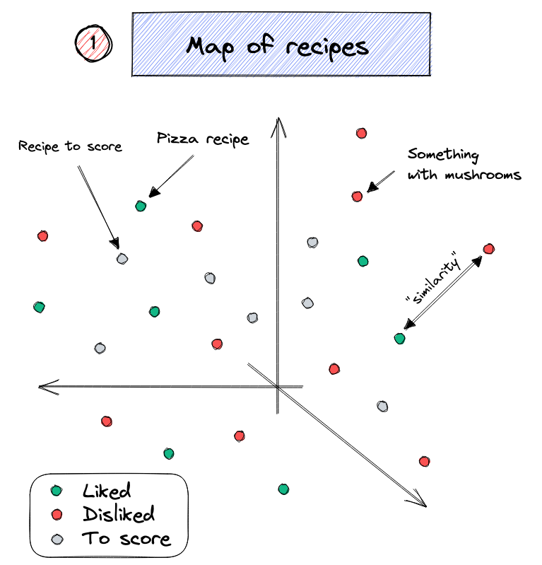
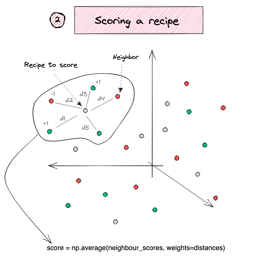
Recipes are the average of the word vectors of the ingredients.

Nearest neighbours used to classify new recipes as potentially delicious.

Analogies with word vectors

Obama is to America as ___ is to Australia.

\text{Obama} - \text{America} + \text{Australia} = ?

wv.most_similar(positive=["Obama", "Australia"], negative=["America"])
[('Mr_Rudd', 0.615142285823822),
 ('Prime_Minister_Julia_Gillard', 0.6045385003089905),
 ('Prime_Minister_Kevin_Rudd', 0.5982581973075867),
 ('Kevin_Rudd', 0.5627648830413818),
 ('Ms_Gillard', 0.5517690181732178),
 ('Opposition_Leader_Kevin_Rudd', 0.5298037528991699),
 ('Mr_Beazley', 0.5259249806404114),
 ('Gillard', 0.5250653028488159),
 ('NARDA_GILMORE', 0.5203536748886108),
 ('Mr_Downer', 0.5150347948074341)]

Testing more associations

wv.most_similar(positive=["France", "London"], negative=["Paris"])
[('Britain', 0.7368934750556946),
 ('UK', 0.6637030839920044),
 ('England', 0.6119861602783203),
 ('United_Kingdom', 0.6067784428596497),
 ('Great_Britain', 0.5870823860168457),
 ('Britian', 0.5852951407432556),
 ('Scotland', 0.5410018563270569),
 ('British', 0.5318331718444824),
 ('Europe', 0.5307437181472778),
 ('East_Midlands', 0.5230222344398499)]

Quickly get to bad associations

wv.most_similar(positive=["King", "woman"], negative=["man"])
[('Queen', 0.5515626072883606),
 ('Oprah_BFF_Gayle', 0.47597548365592957),
 ('Geoffrey_Rush_Exit', 0.46460166573524475),
 ('Princess', 0.4533674418926239),
 ('Yvonne_Stickney', 0.4507041573524475),
 ('L._Bonauto', 0.4422135353088379),
 ('gal_pal_Gayle', 0.4408389925956726),
 ('Alveda_C.', 0.440279096364975),
 ('Tupou_V.', 0.4373863935470581),
 ('K._Letourneau', 0.435103178024292)]
wv.most_similar(positive=["computer_programmer", "woman"], negative=["man"])
[('homemaker', 0.5627118945121765),
 ('housewife', 0.5105047225952148),
 ('graphic_designer', 0.5051802396774292),
 ('schoolteacher', 0.49794942140579224),
 ('businesswoman', 0.493489146232605),
 ('paralegal', 0.4925510883331299),
 ('registered_nurse', 0.4907974898815155),
 ('saleswoman', 0.48816272616386414),
 ('electrical_engineer', 0.4797726571559906),
 ('mechanical_engineer', 0.4755399525165558)]

Bias in NLP models

… there are serious questions to answer, like how are we going to teach AI using public data without incorporating the worst traits of humanity? If we create bots that mirror their users, do we care if their users are human trash? There are plenty of examples of technology embodying — either accidentally or on purpose — the prejudices of society, and Tay’s adventures on Twitter show that even big corporations like Microsoft forget to take any preventative measures against these problems.

The library cheats a little bit

wv.similar_by_vector(wv["computer_programmer"]-wv["man"]+wv["woman"])
[('computer_programmer', 0.910581111907959),
 ('homemaker', 0.5771315693855286),
 ('schoolteacher', 0.5500192046165466),
 ('graphic_designer', 0.5464698672294617),
 ('mechanical_engineer', 0.539836585521698),
 ('electrical_engineer', 0.5337055325508118),
 ('housewife', 0.5274525284767151),
 ('programmer', 0.5096209049224854),
 ('businesswoman', 0.5029540657997131),
 ('keypunch_operator', 0.4974639415740967)]

To get the ‘nice’ analogies, the .most_similar ignores the input words as possible answers.

# ignore (don't return) keys from the input
result = [
    (self.index_to_key[sim + clip_start], float(dists[sim]))
    for sim in best if (sim + clip_start) not in all_keys
]

Car Crash NLP Part II

Predict injury severity

features = df["SUMMARY_EN"]
target = LabelEncoder().fit_transform(df["INJSEVB"])

X_main, X_test, y_main, y_test = \
    train_test_split(features, target, test_size=0.2, random_state=1)
X_train, X_val, y_train, y_val = \
    train_test_split(X_main, y_main, test_size=0.25, random_state=1)
X_train.shape, X_val.shape, X_test.shape
((4169,), (1390,), (1390,))

Using Keras TextVectorization

max_tokens = 1_000
vect = layers.TextVectorization(
    max_tokens=max_tokens,
    output_mode="tf_idf",
    standardize="lower_and_strip_punctuation",
)

vect.adapt(X_train)
vocab = vect.get_vocabulary()

X_train_txt = vect(X_train)
X_val_txt = vect(X_val)
X_test_txt = vect(X_test)

print(vocab[:50])
['[UNK]', 'the', 'was', 'a', 'to', 'of', 'and', 'in', 'driver', 'for', 'this', 'vehicle', 'critical', 'lane', 'he', 'on', 'with', 'that', 'left', 'roadway', 'coded', 'she', 'event', 'crash', 'not', 'at', 'intersection', 'traveling', 'right', 'precrash', 'as', 'from', 'were', 'by', 'had', 'reason', 'his', 'side', 'is', 'front', 'her', 'traffic', 'an', 'it', 'two', 'speed', 'stated', 'one', 'occurred', 'no']

The TF-IDF vectors

pd.DataFrame(X_train_txt, columns=vocab, index=X_train.index)
[UNK] the was a to of and in driver for ... encroaching closely ordinarily locked history fourleg determined box altima above
2532 121.857956 42.274662 10.395409 10.395409 11.785541 8.323526 8.323526 9.775118 3.489896 4.168983 ... 0.0 0.0 0.00000 0.0 0.0 0.0 0.0 0.0 0.0 0.0
6209 72.596230 17.325682 10.395409 5.544218 4.159603 5.549018 7.629900 4.887559 4.187876 6.253474 ... 0.0 0.0 0.00000 0.0 0.0 0.0 0.0 0.0 0.0 0.0
2561 124.450676 30.493198 15.246599 11.088436 9.012472 7.629900 8.323526 2.792891 3.489896 5.558644 ... 0.0 0.0 0.00000 0.0 0.0 0.0 0.0 0.0 0.0 0.0
... ... ... ... ... ... ... ... ... ... ... ... ... ... ... ... ... ... ... ... ... ...
6882 75.188950 20.790817 4.851191 7.623300 9.012472 4.855391 4.161763 2.094668 5.583834 2.084491 ... 0.0 0.0 3.61771 0.0 0.0 0.0 0.0 0.0 0.0 0.0
206 147.785172 27.028063 13.167518 6.237246 8.319205 4.855391 6.242645 2.094668 3.489896 9.032796 ... 0.0 0.0 0.00000 0.0 0.0 0.0 0.0 0.0 0.0 0.0
6356 75.188950 15.246599 9.702381 8.316327 7.625938 5.549018 7.629900 8.378673 2.791917 5.558644 ... 0.0 0.0 0.00000 0.0 0.0 0.0 0.0 0.0 0.0 0.0

4169 rows × 1000 columns

Feed TF-IDF into an ANN

random.seed(42)
tfidf_model = keras.models.Sequential([
    layers.Input((X_train_txt.shape[1],)),
    layers.Dense(250, "relu"),
    layers.Dense(1, "sigmoid")
])

tfidf_model.compile("adam", "binary_crossentropy", metrics=["accuracy"])
tfidf_model.summary()
Model: "sequential_4"
┏━━━━━━━━━━━━━━━━━━━━━━━━━━━━━━━━━┳━━━━━━━━━━━━━━━━━━━━━━━━┳━━━━━━━━━━━━━━━┓
┃ Layer (type)                     Output Shape                  Param # ┃
┡━━━━━━━━━━━━━━━━━━━━━━━━━━━━━━━━━╇━━━━━━━━━━━━━━━━━━━━━━━━╇━━━━━━━━━━━━━━━┩
│ dense_8 (Dense)                 │ (None, 250)            │       250,250 │
├─────────────────────────────────┼────────────────────────┼───────────────┤
│ dense_9 (Dense)                 │ (None, 1)              │           251 │
└─────────────────────────────────┴────────────────────────┴───────────────┘
 Total params: 250,501 (978.52 KB)
 Trainable params: 250,501 (978.52 KB)
 Non-trainable params: 0 (0.00 B)

Fit & evaluate

es = keras.callbacks.EarlyStopping(patience=3, restore_best_weights=True,
    monitor="val_accuracy", verbose=2)

if not Path("tfidf-model.keras").exists():
    tfidf_model.fit(X_train_txt, y_train, epochs=1_000, callbacks=es,
        validation_data=(X_val_txt, y_val), verbose=0)
    tfidf_model.save("tfidf-model.keras")
else:
    tfidf_model = keras.models.load_model("tfidf-model.keras")
tfidf_model.evaluate(X_train_txt, y_train, verbose=0, batch_size=1_000)
[0.06402980536222458, 0.9836891293525696]
tfidf_model.evaluate(X_val_txt, y_val, verbose=0, batch_size=1_000)
[0.33285507559776306, 0.8863309621810913]

Keep text as sequence of tokens

max_length = 500
max_tokens = 1_000
vect = layers.TextVectorization(
    max_tokens=max_tokens,
    output_sequence_length=max_length,
    standardize="lower_and_strip_punctuation",
)

vect.adapt(X_train)
vocab = vect.get_vocabulary()

X_train_txt = vect(X_train)
X_val_txt = vect(X_val)
X_test_txt = vect(X_test)

print(vocab[:50])
['', '[UNK]', 'the', 'was', 'a', 'to', 'of', 'and', 'in', 'driver', 'for', 'this', 'vehicle', 'critical', 'lane', 'he', 'on', 'with', 'that', 'left', 'roadway', 'coded', 'she', 'event', 'crash', 'not', 'at', 'intersection', 'traveling', 'right', 'precrash', 'as', 'from', 'were', 'by', 'had', 'reason', 'his', 'side', 'is', 'front', 'her', 'traffic', 'an', 'it', 'two', 'speed', 'stated', 'one', 'occurred']

A sequence of integers

X_train_txt[0]
tensor([ 11,  24,  49,   8,   2, 253, 219,   6,   4, 165,   8,   2, 410,   6,
          4, 564, 971,  27,   2,  27, 568,   6,   4, 192,   1,  45,  51, 208,
         65, 235,  54,  14,  20, 867,  34,  43, 183,   1,  45,  51, 208,  65,
        235,  54,  14,  20, 178,  34,   4, 676,   1,  42, 237,   2, 153, 192,
         20,   3, 107,   7,  75,  17,   4, 612, 441, 549,   2,  88,  46,   3,
        207,  63, 185,  55,   2,  42, 243,   3, 400,   7,  58,  33,  50, 172,
        251,  84,  26,   2,  60,   6,   2,  24,   1,   4, 402, 970,   1,   1,
          3,  68,  26,   2,  27,  94, 118,   8,  14, 101, 311,  10,   2, 237,
          5, 422, 269,  44, 154,  54,  19,   1,   4, 308, 342,   1,   3,  79,
          8,  14,  45, 159,   2, 121,  27, 190,  44, 598,   5, 325,  75,  70,
          2, 105, 189, 231,   1, 241,  81,  19,  31,   1, 193,   2,  54,  81,
          9, 134,   4, 174,  12,  17,   1, 390,   1, 159,   2,  27,  32,   2,
        119,   1,  68,   8,   2, 410,   6,   2,  27,   8,   1,   5,   2, 159,
        174,  12,   1, 168,   2,  27,   7,  69,   2,  40,   6,   1,  17,  81,
         40,  19, 246,  73,  83,  64,   5, 129,  56,   8,   2,  27,   7,  33,
         73,  71,  57,   5,  82,   2,   9,   6,   1,   4,   1,  59, 382,   5,
        113,   8, 276, 258,   1, 317, 928, 284,  10, 784, 294, 462, 483,   7,
          1,  15,   3,  16,  37, 112,   5, 677, 144,   1,  26,   2,  60,   6,
          2,  24,  15,  47,  18,  70,   2, 105, 429,  15,  35, 448,   1,   5,
        493,  37,  54,  62,  68,  25,   1,  33,   5, 325,  70,  15, 134,   2,
        174, 232, 406,  15, 341, 134,   1, 691,   2,  27,   7,  15,   1,  10,
         93,  15,   3,  25, 216,   8,   2,  24,   2,  13,  30,  23,  10,   1,
          3,  21,  11,  12,  28,  76,   2,  14, 130,  19,  38,   6, 106,  14,
          2,  13,  36,   3,  21,  31,   4,   9,  91, 180,   1, 137,   1,   2,
         87,  97,  21,   5,   1, 285,  43,   1, 511, 569,  15, 775, 140,   1,
          2,  27,   7,  25,  68,  31, 184,  31,   2, 159, 174,  12,   1,   2,
         42,   1,   2,   9,   6,   1,   4,   1,  59,   8, 276, 258,   3, 489,
         37, 753, 544,  10,   4, 975, 313,  26,   2,  60,   6,   2,  24,  15,
          3,  16,  37, 112, 110,  32, 151,  70,   2,  24,  49,  15,  47,  15,
          3,  79,   8,  14, 191,  31,   2,  42, 105, 189, 231,  15, 647,   2,
         12,   8,   2,  19,  94, 118,  35,   1,   5,  54,  19,   7, 141,   2,
         27,  15,   1,  31,   2,  12, 347,  81,  54,   7,  90,   8,   2, 410,
          6,   2,  27,  15, 503,  62, 154,  25, 143,   1,  15, 157, 134,   2,
        174,  12,  17,  81, 390,   7,   1,  16, 111,  15, 168,   2,  27,  15,
        588, 329, 117,   7,   3, 163,   5, 113, 947, 175,  26,   4, 643,   1,
          2,  13,  30,  23,  10,   1,   3,  21,  52,  12])
Feed LSTM a sequence of one-hots

random.seed(42)
inputs = keras.Input(shape=(max_length,), dtype="int64")
onehot = keras.ops.one_hot(inputs, max_tokens)
x = layers.Bidirectional(layers.LSTM(24))(onehot)
x = layers.Dropout(0.5)(x) 
outputs = layers.Dense(1, activation="sigmoid")(x)    
one_hot_model = keras.Model(inputs, outputs)
one_hot_model.compile(optimizer="adam",
    loss="binary_crossentropy", metrics=["accuracy"])
one_hot_model.summary()
Model: "functional_8"
┏━━━━━━━━━━━━━━━━━━━━━━━━━━━━━━━━━┳━━━━━━━━━━━━━━━━━━━━━━━━┳━━━━━━━━━━━━━━━┓
┃ Layer (type)                     Output Shape                  Param # ┃
┡━━━━━━━━━━━━━━━━━━━━━━━━━━━━━━━━━╇━━━━━━━━━━━━━━━━━━━━━━━━╇━━━━━━━━━━━━━━━┩
│ input_layer_5 (InputLayer)      │ (None, 500)            │             0 │
├─────────────────────────────────┼────────────────────────┼───────────────┤
│ one_hot (OneHot)                │ (None, 500, 1000)      │             0 │
├─────────────────────────────────┼────────────────────────┼───────────────┤
│ bidirectional (Bidirectional)   │ (None, 48)             │       196,800 │
├─────────────────────────────────┼────────────────────────┼───────────────┤
│ dropout (Dropout)               │ (None, 48)             │             0 │
├─────────────────────────────────┼────────────────────────┼───────────────┤
│ dense_10 (Dense)                │ (None, 1)              │            49 │
└─────────────────────────────────┴────────────────────────┴───────────────┘
 Total params: 196,849 (768.94 KB)
 Trainable params: 196,849 (768.94 KB)
 Non-trainable params: 0 (0.00 B)

Fit & evaluate

es = keras.callbacks.EarlyStopping(patience=3, restore_best_weights=True,
    monitor="val_accuracy", verbose=2)

# if not Path("one-hot-model.keras").exists():
one_hot_model.fit(X_train_txt, y_train, epochs=1_000, callbacks=es,
    validation_data=(X_val_txt, y_val), verbose=0);
one_hot_model.save("one-hot-model.keras")
# else:
#     one_hot_model = keras.models.load_model("one-hot-model.keras")
Epoch 6: early stopping
Restoring model weights from the end of the best epoch: 3.
one_hot_model.evaluate(X_train_txt, y_train, verbose=0, batch_size=1_000)
[0.5324524641036987, 0.7255936861038208]
one_hot_model.evaluate(X_val_txt, y_val, verbose=0, batch_size=1_000)
[0.5648519992828369, 0.7187050580978394]

Custom embeddings

inputs = keras.Input(shape=(max_length,), dtype="int64")
embedded = layers.Embedding(input_dim=max_tokens, output_dim=32,
        mask_zero=True)(inputs)
x = layers.Bidirectional(layers.LSTM(24))(embedded)
x = layers.Dropout(0.5)(x)
outputs = layers.Dense(1, activation="sigmoid")(x)
embed_lstm = keras.Model(inputs, outputs)
embed_lstm.compile("adam", "binary_crossentropy", metrics=["accuracy"])
embed_lstm.summary()
Model: "functional_10"
┏━━━━━━━━━━━━━━━━━━━━━┳━━━━━━━━━━━━━━━━━━━┳━━━━━━━━━━━━┳━━━━━━━━━━━━━━━━━━━┓
┃ Layer (type)         Output Shape          Param #  Connected to      ┃
┡━━━━━━━━━━━━━━━━━━━━━╇━━━━━━━━━━━━━━━━━━━╇━━━━━━━━━━━━╇━━━━━━━━━━━━━━━━━━━┩
│ input_layer_6       │ (None, 500)       │          0 │ -                 │
│ (InputLayer)        │                   │            │                   │
├─────────────────────┼───────────────────┼────────────┼───────────────────┤
│ embedding           │ (None, 500, 32)   │     32,000 │ input_layer_6[0]… │
│ (Embedding)         │                   │            │                   │
├─────────────────────┼───────────────────┼────────────┼───────────────────┤
│ not_equal           │ (None, 500)       │          0 │ input_layer_6[0]… │
│ (NotEqual)          │                   │            │                   │
├─────────────────────┼───────────────────┼────────────┼───────────────────┤
│ bidirectional_1     │ (None, 48)        │     10,944 │ embedding[0][0],  │
│ (Bidirectional)     │                   │            │ not_equal[0][0]   │
├─────────────────────┼───────────────────┼────────────┼───────────────────┤
│ dropout_1 (Dropout) │ (None, 48)        │          0 │ bidirectional_1[ │
├─────────────────────┼───────────────────┼────────────┼───────────────────┤
│ dense_11 (Dense)    │ (None, 1)         │         49 │ dropout_1[0][0]   │
└─────────────────────┴───────────────────┴────────────┴───────────────────┘
 Total params: 42,993 (167.94 KB)
 Trainable params: 42,993 (167.94 KB)
 Non-trainable params: 0 (0.00 B)

Fit & evaluate

es = keras.callbacks.EarlyStopping(patience=3, restore_best_weights=True,
    monitor="val_accuracy", verbose=2)

# if not Path("embed-lstm.keras").exists():
embed_lstm.fit(X_train_txt, y_train, epochs=1_000, callbacks=es,
    validation_data=(X_val_txt, y_val), verbose=0);
embed_lstm.save("embed-lstm.keras")
# else:
#     embed_lstm = keras.models.load_model("embed-lstm.keras")
Epoch 13: early stopping
Restoring model weights from the end of the best epoch: 10.
embed_lstm.evaluate(X_train_txt, y_train, verbose=0, batch_size=1_000)
[0.2964944839477539, 0.8848644495010376]
embed_lstm.evaluate(X_val_txt, y_val, verbose=0, batch_size=1_000)
[0.3567287027835846, 0.8712230324745178]
embed_lstm.evaluate(X_test_txt, y_test, verbose=0, batch_size=1_000)
[0.36198052763938904, 0.8647481799125671]

Package Versions

from watermark import watermark
print(watermark(python=True, packages="keras,matplotlib,numpy,pandas,seaborn,scipy,torch,tensorflow,tf_keras"))
Python implementation: CPython
Python version       : 3.11.8
IPython version      : 8.23.0

keras     : 3.2.0
matplotlib: 3.8.4
numpy     : 1.26.4
pandas    : 2.2.1
seaborn   : 0.13.2
scipy     : 1.11.0
torch     : 2.2.2
tensorflow: 2.16.1
tf_keras  : 2.16.0

Glossary

  • bag of words
  • lemmatization
  • n-grams
  • one-hot embedding
  • permutation importance test
  • TF-IDF
  • vocabulary
  • word embedding
  • word2vec