Recurrent Neural Networks

ACTL3143 & ACTL5111 Deep Learning for Actuaries

Patrick Laub

Tensors & Time Series

Lecture Outline

• Tensors & Time Series

• Some Recurrent Structures

• Recurrent Neural Networks

• CoreLogic Hedonic Home Value Index

• Splitting time series data

• Predicting Sydney House Prices

• Predicting Multiple Time Series

Shapes of data

Illustration of tensors of different rank.

The axis argument in numpy

Starting with a (3, 4)-shaped matrix:

X = np.arange(12).reshape(3,4)
X

array([[ 0,  1,  2,  3],
       [ 4,  5,  6,  7],
       [ 8,  9, 10, 11]])

axis=0: (3, 4) \leadsto (4,).

X.sum(axis=0)

array([12, 15, 18, 21])

axis=1: (3, 4) \leadsto (3,).

X.prod(axis=1)

array([   0,  840, 7920])

The return value’s rank is one less than the input’s rank.

Important

The axis parameter tells us which dimension is removed.

Using axis & keepdims

With keepdims=True, the rank doesn’t change.

X = np.arange(12).reshape(3,4)
X

array([[ 0,  1,  2,  3],
       [ 4,  5,  6,  7],
       [ 8,  9, 10, 11]])

axis=0: (3, 4) \leadsto (1, 4).

X.sum(axis=0, keepdims=True)

array([[12, 15, 18, 21]])

axis=1: (3, 4) \leadsto (3, 1).

X.prod(axis=1, keepdims=True)

array([[   0],
       [ 840],
       [7920]])

X / X.sum(axis=1)

ValueError: operands could not be broadcast together with shapes (3,4) (3,) 

X / X.sum(axis=1, keepdims=True)

array([[0.  , 0.17, 0.33, 0.5 ],
       [0.18, 0.23, 0.27, 0.32],
       [0.21, 0.24, 0.26, 0.29]])

The rank of a time series

Say we had n observations of a time series x_1, x_2, \dots, x_n.

This \mathbf{x} = (x_1, \dots, x_n) would have shape (n,) & rank 1.

If instead we had a batch of b time series’

\mathbf{X} = \begin{pmatrix} x_7 & x_8 & \dots & x_{7+n-1} \\ x_2 & x_3 & \dots & x_{2+n-1} \\ \vdots & \vdots & \ddots & \vdots \\ x_3 & x_4 & \dots & x_{3+n-1} \\ \end{pmatrix} \,,

the batch \mathbf{X} would have shape (b, n) & rank 2.

Multivariate time series

t	x	y
0	x_0	y_0
1	x_1	y_1
2	x_2	y_2
3	x_3	y_3

Say n observations of the m time series, would be a shape (n, m) matrix of rank 2.

In Keras, a batch of b of these time series has shape (b, n, m) and has rank 3.

Note

Use \mathbf{x}_t \in \mathbb{R}^{1 \times m} to denote the vector of all time series at time t. Here, \mathbf{x}_t = (x_t, y_t).

Some Recurrent Structures

Lecture Outline

• Tensors & Time Series

• Some Recurrent Structures

• Recurrent Neural Networks

• CoreLogic Hedonic Home Value Index

• Splitting time series data

• Predicting Sydney House Prices

• Predicting Multiple Time Series

Recurrence relation

A recurrence relation is an equation that expresses each element of a sequence as a function of the preceding ones. More precisely, in the case where only the immediately preceding element is involved, a recurrence relation has the form

u_n = \psi(n, u_{n-1}) \quad \text{ for } \quad n > 0.

Example: Factorial n! = n (n-1)! for n > 0 given 0! = 1.

Diagram of an RNN cell

The RNN processes each data in the sequence one by one, while keeping memory of what came before.

Schematic of a simple recurrent neural network. E.g. SimpleRNN, LSTM, or GRU.

A SimpleRNN cell.

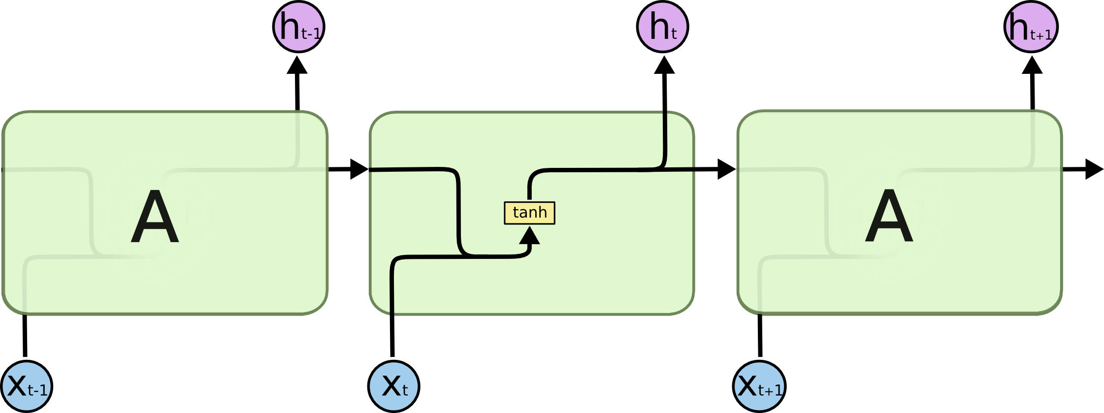
Diagram of a SimpleRNN cell.

All the outputs before the final one are often discarded.

SimpleRNN

Say each prediction is a vector of size d, so \mathbf{y}_t \in \mathbb{R}^{1 \times d}.

Then the main equation of a SimpleRNN, given \mathbf{y}_0 = \mathbf{0}, is

\mathbf{y}_t = \psi\bigl( \mathbf{x}_t \mathbf{W}_x + \mathbf{y}_{t-1} \mathbf{W}_y + \mathbf{b} \bigr) .

Here, \begin{aligned} &\mathbf{x}_t \in \mathbb{R}^{1 \times m}, \mathbf{W}_x \in \mathbb{R}^{m \times d}, \\ &\mathbf{y}_{t-1} \in \mathbb{R}^{1 \times d}, \mathbf{W}_y \in \mathbb{R}^{d \times d}, \text{ and } \mathbf{b} \in \mathbb{R}^{d}. \end{aligned}

SimpleRNN (in batches)

Say we operate on batches of size b, then \mathbf{Y}_t \in \mathbb{R}^{b \times d}.

The main equation of a SimpleRNN, given \mathbf{Y}_0 = \mathbf{0}, is \mathbf{Y}_t = \psi\bigl( \mathbf{X}_t \mathbf{W}_x + \mathbf{Y}_{t-1} \mathbf{W}_y + \mathbf{b} \bigr) . Here, \begin{aligned} &\mathbf{X}_t \in \mathbb{R}^{b \times m}, \mathbf{W}_x \in \mathbb{R}^{m \times d}, \\ &\mathbf{Y}_{t-1} \in \mathbb{R}^{b \times d}, \mathbf{W}_y \in \mathbb{R}^{d \times d}, \text{ and } \mathbf{b} \in \mathbb{R}^{d}. \end{aligned}

Simple Keras demo

num_obs = 4
num_time_steps = 3
num_time_series = 2

X = np.arange(num_obs*num_time_steps*num_time_series).astype(np.float32) \
        .reshape([num_obs, num_time_steps, num_time_series])

output_size = 1                                                                 
y = np.array([0, 0, 1, 1])

X[:2]

array([[[ 0.,  1.],
        [ 2.,  3.],
        [ 4.,  5.]],

       [[ 6.,  7.],
        [ 8.,  9.],
        [10., 11.]]], dtype=float32)

X[2:]

array([[[12., 13.],
        [14., 15.],
        [16., 17.]],

       [[18., 19.],
        [20., 21.],
        [22., 23.]]], dtype=float32)

Keras’ SimpleRNN

As usual, the SimpleRNN is just a layer in Keras.

from keras.layers import SimpleRNN

random.seed(1234)
model = Sequential([
  SimpleRNN(output_size, activation="sigmoid")
])
model.compile(loss="binary_crossentropy", metrics=["accuracy"])

hist = model.fit(X, y, epochs=500, verbose=False)
model.evaluate(X, y, verbose=False)

[3.1845884323120117, 0.5]

The predicted probabilities on the training set are:

model.predict(X, verbose=0)

array([[0.97],
       [1.  ],
       [1.  ],
       [1.  ]], dtype=float32)

SimpleRNN weights

model.get_weights()

[array([[0.68],
        [0.21]], dtype=float32),
 array([[0.49]], dtype=float32),
 array([-0.51], dtype=float32)]

def sigmoid(x):
  return 1 / (1 + np.exp(-x))

W_x, W_y, b = model.get_weights()

Y = np.zeros((num_obs, output_size), dtype=np.float32)
for t in range(num_time_steps):
    X_t = X[:, t, :]
    z = X_t @ W_x + Y @ W_y + b
    Y = sigmoid(z)

Y

array([[0.97],
       [1.  ],
       [1.  ],
       [1.  ]], dtype=float32)

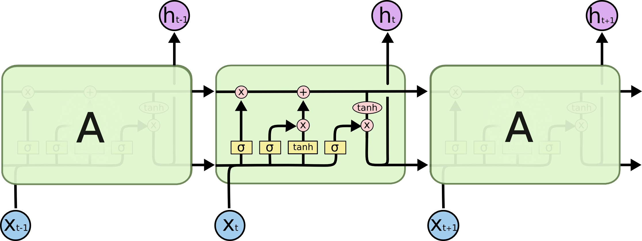
LSTM internals

GRU internals

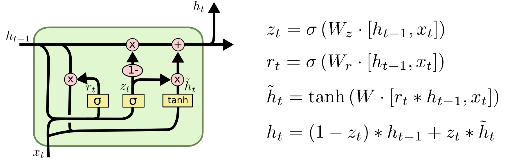
Diagram of a GRU cell.

Recurrent Neural Networks

Lecture Outline

• Tensors & Time Series

• Some Recurrent Structures

• Recurrent Neural Networks

• CoreLogic Hedonic Home Value Index

• Splitting time series data

• Predicting Sydney House Prices

• Predicting Multiple Time Series

Basic facts of RNNs

• A recurrent neural network is a type of neural network that is designed to process sequences of data (e.g. time series, sentences).
• A recurrent neural network is any network that contains a recurrent layer.
• A recurrent layer is a layer that processes data in a sequence.
• An RNN can have one or more recurrent layers.
• Weights are shared over time; this allows the model to be used on arbitrary-length sequences.

Applications

• Forecasting: revenue forecast, weather forecast, predict disease rate from medical history, etc.
• Classification: given a time series of the activities of a visitor on a website, classify whether the visitor is a bot or a human.
• Event detection: given a continuous data stream, identify the occurrence of a specific event. Example: Detect utterances like “Hey Alexa” from an audio stream.
• Anomaly detection: given a continuous data stream, detect anything unusual happening. Example: Detect unusual activity on the corporate network.

Input and output sequences

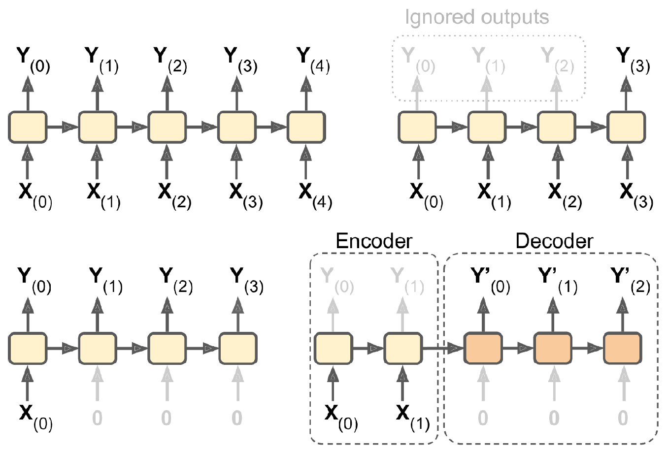
Categories of recurrent neural networks: sequence to sequence, sequence to vector, vector to sequence, encoder-decoder network.

Input and output sequences

• Sequence to sequence: Useful for predicting time series such as using prices over the last N days to output the prices shifted one day into the future (i.e. from N-1 days ago to tomorrow.)
• Sequence to vector: ignore all outputs in the previous time steps except for the last one. Example: give a sentiment score to a sequence of words corresponding to a movie review.

Input and output sequences

• Vector to sequence: feed the network the same input vector over and over at each time step and let it output a sequence. Example: given that the input is an image, find a caption for it. The image is treated as an input vector (pixels in an image do not follow a sequence). The caption is a sequence of textual description of the image. A dataset containing images and their descriptions is the input of the RNN.
• The Encoder-Decoder: The encoder is a sequence-to-vector network. The decoder is a vector-to-sequence network. Example: Feed the network a sequence in one language. Use the encoder to convert the sentence into a single vector representation. The decoder decodes this vector into the translation of the sentence in another language.

Recurrent layers can be stacked.

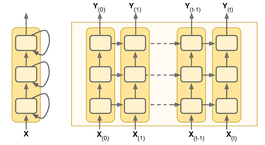
Deep RNN unrolled through time.

CoreLogic Hedonic Home Value Index

Lecture Outline

• Tensors & Time Series

• Some Recurrent Structures

• Recurrent Neural Networks

• CoreLogic Hedonic Home Value Index

• Splitting time series data

• Predicting Sydney House Prices

• Predicting Multiple Time Series

Australian House Price Indices

Percentage changes

changes = house_prices.pct_change().dropna()
changes.round(2)

	Brisbane	East_Bris	North_Bris	West_Bris	Melbourne	North_Syd	Sydney
Date
1990-02-28	0.03	-0.01	0.01	0.01	0.00	-0.00	-0.02
1990-03-31	0.01	0.03	0.01	0.01	0.02	-0.00	0.03
...	...	...	...	...	...	...	...
2021-04-30	0.03	0.01	0.01	-0.00	0.01	0.02	0.02
2021-05-31	0.03	0.03	0.03	0.03	0.03	0.02	0.04

376 rows × 7 columns

Percentage changes

changes.plot();

The size of the changes

changes.mean()

Brisbane      0.005496
East_Bris     0.005416
North_Bris    0.005024
West_Bris     0.004842
Melbourne     0.005677
North_Syd     0.004819
Sydney        0.005526
dtype: float64

changes *= 100

changes.mean()

Brisbane      0.549605
East_Bris     0.541562
North_Bris    0.502390
West_Bris     0.484204
Melbourne     0.567700
North_Syd     0.481863
Sydney        0.552641
dtype: float64

changes.plot(legend=False);

Splitting time series data

Lecture Outline

• Tensors & Time Series

• Some Recurrent Structures

• Recurrent Neural Networks

• CoreLogic Hedonic Home Value Index

• Splitting time series data

• Predicting Sydney House Prices

• Predicting Multiple Time Series

Split without shuffling

num_train = int(0.6 * len(changes))
num_val = int(0.2 * len(changes))
num_test = len(changes) - num_train - num_val
print(f"# Train: {num_train}, # Val: {num_val}, # Test: {num_test}")

# Train: 225, # Val: 75, # Test: 76

Subsequences of a time series

Keras has a built-in method for converting a time series into subsequences/chunks.

from keras.utils import timeseries_dataset_from_array

integers = range(10)                                
dummy_dataset = timeseries_dataset_from_array(
    data=integers[:-3],                                 
    targets=integers[3:],                               
    sequence_length=3,                                      
    batch_size=2,                                           
)

for inputs, targets in dummy_dataset:
    for i in range(inputs.shape[0]):
        print([int(x) for x in inputs[i]], int(targets[i]))

[0, 1, 2] 3
[1, 2, 3] 4
[2, 3, 4] 5
[3, 4, 5] 6
[4, 5, 6] 7

On time series splits

If you have a lot of time series data, then use:

from keras.utils import timeseries_dataset_from_array
data = range(20); seq = 3; ts = data[:-seq]; target = data[seq:]
nTrain = int(0.5 * len(ts)); nVal = int(0.25 * len(ts))
nTest = len(ts) - nTrain - nVal
print(f"# Train: {nTrain}, # Val: {nVal}, # Test: {nTest}")

# Train: 8, # Val: 4, # Test: 5

trainDS = \
  timeseries_dataset_from_array(
    ts, target, seq,
    end_index=nTrain)

valDS = \
  timeseries_dataset_from_array(
    ts, target, seq,
    start_index=nTrain,
    end_index=nTrain+nVal)

testDS = \
  timeseries_dataset_from_array(
    ts, target, seq,
    start_index=nTrain+nVal)

Training dataset
[0, 1, 2] 3
[1, 2, 3] 4
[2, 3, 4] 5
[3, 4, 5] 6
[4, 5, 6] 7
[5, 6, 7] 8

Validation dataset
[8, 9, 10] 11
[9, 10, 11] 12

Test dataset
[12, 13, 14] 15
[13, 14, 15] 16
[14, 15, 16] 17

On time series splits II

If you don’t have a lot of time series data, consider:

X = []; y = []
for i in range(len(data)-seq):
    X.append(data[i:i+seq])
    y.append(data[i+seq])
X = np.array(X); y = np.array(y);

nTrain = int(0.5 * X.shape[0])
X_train = X[:nTrain]
y_train = y[:nTrain]

nVal = int(np.ceil(0.25 * X.shape[0]))
X_val = X[nTrain:nTrain+nVal]
y_val = y[nTrain:nTrain+nVal]

nTest = X.shape[0] - nTrain - nVal
X_test = X[nTrain+nVal:]
y_test = y[nTrain+nVal:]

Training dataset
[0, 1, 2] 3
[1, 2, 3] 4
[2, 3, 4] 5
[3, 4, 5] 6
[4, 5, 6] 7
[5, 6, 7] 8
[6, 7, 8] 9
[7, 8, 9] 10

Validation dataset
[8, 9, 10] 11
[9, 10, 11] 12
[10, 11, 12] 13
[11, 12, 13] 14
[12, 13, 14] 15

Test dataset
[13, 14, 15] 16
[14, 15, 16] 17
[15, 16, 17] 18
[16, 17, 18] 19

Predicting Sydney House Prices

Lecture Outline

• Tensors & Time Series

• Some Recurrent Structures

• Recurrent Neural Networks

• CoreLogic Hedonic Home Value Index

• Splitting time series data

• Predicting Sydney House Prices

• Predicting Multiple Time Series

Creating dataset objects

# Num. of input time series.
num_ts = changes.shape[1]

# How many prev. months to use.
seq_length = 6

# Predict the next month ahead.
ahead = 1

# The index of the first target.
delay = (seq_length+ahead-1)

# Which suburb to predict.
target_suburb = changes["Sydney"]

train_ds = \
  timeseries_dataset_from_array(
    changes[:-delay],
    targets=target_suburb[delay:],
    sequence_length=seq_length,
    end_index=num_train)

val_ds = \
  timeseries_dataset_from_array(
    changes[:-delay],
    targets=target_suburb[delay:],
    sequence_length=seq_length,
    start_index=num_train,
    end_index=num_train+num_val)

test_ds = \
  timeseries_dataset_from_array(
    changes[:-delay],
    targets=target_suburb[delay:],
    sequence_length=seq_length,
    start_index=num_train+num_val)

Converting Dataset to numpy

The Dataset object can be handed to Keras directly, but if we really need a numpy array, we can run:

X_train = np.concatenate(list(train_ds.map(lambda x, y: x)))
y_train = np.concatenate(list(train_ds.map(lambda x, y: y)))

The shape of our training set is now:

X_train.shape

(220, 6, 7)

y_train.shape

(220,)

Converting the rest to numpy arrays:

X_val = np.concatenate(list(val_ds.map(lambda x, y: x)))
y_val = np.concatenate(list(val_ds.map(lambda x, y: y)))
X_test = np.concatenate(list(test_ds.map(lambda x, y: x)))
y_test = np.concatenate(list(test_ds.map(lambda x, y: y)))

A dense network

from keras.layers import Input, Flatten
random.seed(1)
model_dense = Sequential([
    Input((seq_length, num_ts)),
    Flatten(),
    Dense(50, activation="leaky_relu"),
    Dense(20, activation="leaky_relu"),
    Dense(1, activation="linear")
])
model_dense.compile(loss="mse", optimizer="adam")
print(f"This model has {model_dense.count_params()} parameters.")

es = EarlyStopping(patience=50, restore_best_weights=True, verbose=1)
%time hist = model_dense.fit(X_train, y_train, epochs=1_000, \
  validation_data=(X_val, y_val), callbacks=[es], verbose=0);

This model has 3191 parameters.
Epoch 57: early stopping
Restoring model weights from the end of the best epoch: 7.
CPU times: user 2.92 s, sys: 267 ms, total: 3.18 s
Wall time: 2.84 s

Plot the model

from keras.utils import plot_model
plot_model(model_dense, show_shapes=True)

Assess the fits

model_dense.evaluate(X_val, y_val, verbose=0)

1.1644608974456787

Plotting the predictions

A SimpleRNN layer

random.seed(1)

model_simple = Sequential([
    Input((seq_length, num_ts)),
    SimpleRNN(50),
    Dense(1, activation="linear")
])
model_simple.compile(loss="mse", optimizer="adam")
print(f"This model has {model_simple.count_params()} parameters.")

es = EarlyStopping(patience=50, restore_best_weights=True, verbose=1)
%time hist = model_simple.fit(X_train, y_train, epochs=1_000, \
  validation_data=(X_val, y_val), callbacks=[es], verbose=0);

This model has 2951 parameters.
Epoch 62: early stopping
Restoring model weights from the end of the best epoch: 12.
CPU times: user 3.77 s, sys: 452 ms, total: 4.22 s
Wall time: 3.23 s

Assess the fits

model_simple.evaluate(X_val, y_val, verbose=0)

1.2507916688919067

Plot the model

plot_model(model_simple, show_shapes=True)

Plotting the predictions

WARNING:tensorflow:5 out of the last 7 calls to <function TensorFlowTrainer.make_predict_function.<locals>.one_step_on_data_distributed at 0x7a2c503049a0> triggered tf.function retracing. Tracing is expensive and the excessive number of tracings could be due to (1) creating @tf.function repeatedly in a loop, (2) passing tensors with different shapes, (3) passing Python objects instead of tensors. For (1), please define your @tf.function outside of the loop. For (2), @tf.function has reduce_retracing=True option that can avoid unnecessary retracing. For (3), please refer to https://www.tensorflow.org/guide/function#controlling_retracing and https://www.tensorflow.org/api_docs/python/tf/function for  more details.

A LSTM layer

from keras.layers import LSTM

random.seed(1)

model_lstm = Sequential([
    Input((seq_length, num_ts)),
    LSTM(50),
    Dense(1, activation="linear")
])

model_lstm.compile(loss="mse", optimizer="adam")

es = EarlyStopping(patience=50, restore_best_weights=True, verbose=1)

%time hist = model_lstm.fit(X_train, y_train, epochs=1_000, \
  validation_data=(X_val, y_val), callbacks=[es], verbose=0);

Epoch 59: early stopping
Restoring model weights from the end of the best epoch: 9.
CPU times: user 4.5 s, sys: 442 ms, total: 4.94 s
Wall time: 3.73 s

Assess the fits

model_lstm.evaluate(X_val, y_val, verbose=0)

0.8353261947631836

Plotting the predictions

WARNING:tensorflow:6 out of the last 8 calls to <function TensorFlowTrainer.make_predict_function.<locals>.one_step_on_data_distributed at 0x7a2c882e79c0> triggered tf.function retracing. Tracing is expensive and the excessive number of tracings could be due to (1) creating @tf.function repeatedly in a loop, (2) passing tensors with different shapes, (3) passing Python objects instead of tensors. For (1), please define your @tf.function outside of the loop. For (2), @tf.function has reduce_retracing=True option that can avoid unnecessary retracing. For (3), please refer to https://www.tensorflow.org/guide/function#controlling_retracing and https://www.tensorflow.org/api_docs/python/tf/function for  more details.

A GRU layer

from keras.layers import GRU

random.seed(1)

model_gru = Sequential([
    Input((seq_length, num_ts)),
    GRU(50),
    Dense(1, activation="linear")
])

model_gru.compile(loss="mse", optimizer="adam")

es = EarlyStopping(patience=50, restore_best_weights=True, verbose=1)

%time hist = model_gru.fit(X_train, y_train, epochs=1_000, \
  validation_data=(X_val, y_val), callbacks=[es], verbose=0)

Epoch 57: early stopping
Restoring model weights from the end of the best epoch: 7.
CPU times: user 4.71 s, sys: 530 ms, total: 5.24 s
Wall time: 3.76 s

Assess the fits

model_gru.evaluate(X_val, y_val, verbose=0)

0.7435100674629211

Plotting the predictions

Two GRU layers

random.seed(1)

model_two_grus = Sequential([
    Input((seq_length, num_ts)),
    GRU(50, return_sequences=True),
    GRU(50),
    Dense(1, activation="linear")
])

model_two_grus.compile(loss="mse", optimizer="adam")

es = EarlyStopping(patience=50, restore_best_weights=True, verbose=1)

%time hist = model_two_grus.fit(X_train, y_train, epochs=1_000, \
  validation_data=(X_val, y_val), callbacks=[es], verbose=0)

Epoch 56: early stopping
Restoring model weights from the end of the best epoch: 6.
CPU times: user 7.44 s, sys: 818 ms, total: 8.25 s
Wall time: 9.19 s

Assess the fits

model_two_grus.evaluate(X_val, y_val, verbose=0)

0.7989509105682373

Plotting the predictions

Compare the models

	Model	MSE
1	SimpleRNN	1.250792
0	Dense	1.164461
2	LSTM	0.835326
4	2 GRUs	0.798951
3	GRU	0.743510

The network with two GRU layers is the best.

model_two_grus.evaluate(test_ds, verbose=0)

1.8552547693252563

Test set

Predicting Multiple Time Series

Lecture Outline

• Tensors & Time Series

• Some Recurrent Structures

• Recurrent Neural Networks

• CoreLogic Hedonic Home Value Index

• Splitting time series data

• Predicting Sydney House Prices

• Predicting Multiple Time Series

Creating dataset objects

Change the targets argument to include all the suburbs.

train_ds = \
  timeseries_dataset_from_array(
    changes[:-delay],
    targets=changes[delay:],
    sequence_length=seq_length,
    end_index=num_train)

val_ds = \
  timeseries_dataset_from_array(
    changes[:-delay],
    targets=changes[delay:],
    sequence_length=seq_length,
    start_index=num_train,
    end_index=num_train+num_val)

test_ds = \
  timeseries_dataset_from_array(
    changes[:-delay],
    targets=changes[delay:],
    sequence_length=seq_length,
    start_index=num_train+num_val)

Converting Dataset to numpy

The shape of our training set is now:

X_train = np.concatenate(list(train_ds.map(lambda x, y: x)))
X_train.shape

(220, 6, 7)

y_train = np.concatenate(list(train_ds.map(lambda x, y: y)))
y_train.shape

(220, 7)

Converting the rest to numpy arrays:

X_val = np.concatenate(list(val_ds.map(lambda x, y: x)))
y_val = np.concatenate(list(val_ds.map(lambda x, y: y)))
X_test = np.concatenate(list(test_ds.map(lambda x, y: x)))
y_test = np.concatenate(list(test_ds.map(lambda x, y: y)))

A dense network

random.seed(1)
model_dense = Sequential([
    Input((seq_length, num_ts)),
    Flatten(),
    Dense(50, activation="leaky_relu"),
    Dense(20, activation="leaky_relu"),
    Dense(num_ts, activation="linear")
])
model_dense.compile(loss="mse", optimizer="adam")
print(f"This model has {model_dense.count_params()} parameters.")

es = EarlyStopping(patience=50, restore_best_weights=True, verbose=1)
%time hist = model_dense.fit(X_train, y_train, epochs=1_000, \
  validation_data=(X_val, y_val), callbacks=[es], verbose=0);

This model has 3317 parameters.
Epoch 75: early stopping
Restoring model weights from the end of the best epoch: 25.
CPU times: user 3.6 s, sys: 338 ms, total: 3.93 s
Wall time: 6.72 s

Plot the model

plot_model(model_dense, show_shapes=True)

Assess the fits

model_dense.evaluate(X_val, y_val, verbose=0)

1.4294650554656982

Plotting the predictions

A SimpleRNN layer

random.seed(1)

model_simple = Sequential([
    Input((seq_length, num_ts)),
    SimpleRNN(50),
    Dense(num_ts, activation="linear")
])
model_simple.compile(loss="mse", optimizer="adam")
print(f"This model has {model_simple.count_params()} parameters.")

es = EarlyStopping(patience=50, restore_best_weights=True, verbose=1)
%time hist = model_simple.fit(X_train, y_train, epochs=1_000, \
  validation_data=(X_val, y_val), callbacks=[es], verbose=0);

This model has 3257 parameters.
Epoch 70: early stopping
Restoring model weights from the end of the best epoch: 20.
CPU times: user 4.18 s, sys: 391 ms, total: 4.57 s
Wall time: 6.02 s

Assess the fits

model_simple.evaluate(X_val, y_val, verbose=0)

1.4916820526123047

Plot the model

plot_model(model_simple, show_shapes=True)

Plotting the predictions

A LSTM layer

random.seed(1)

model_lstm = Sequential([
    Input((seq_length, num_ts)),
    LSTM(50),
    Dense(num_ts, activation="linear")
])

model_lstm.compile(loss="mse", optimizer="adam")

es = EarlyStopping(patience=50, restore_best_weights=True, verbose=1)

%time hist = model_lstm.fit(X_train, y_train, epochs=1_000, \
  validation_data=(X_val, y_val), callbacks=[es], verbose=0);

Epoch 74: early stopping
Restoring model weights from the end of the best epoch: 24.
CPU times: user 4.5 s, sys: 371 ms, total: 4.87 s
Wall time: 3.57 s

Assess the fits

model_lstm.evaluate(X_val, y_val, verbose=0)

1.3311247825622559

Plotting the predictions

A GRU layer

random.seed(1)

model_gru = Sequential([
    Input((seq_length, num_ts)),
    GRU(50),
    Dense(num_ts, activation="linear")
])

model_gru.compile(loss="mse", optimizer="adam")

es = EarlyStopping(patience=50, restore_best_weights=True, verbose=1)

%time hist = model_gru.fit(X_train, y_train, epochs=1_000, \
  validation_data=(X_val, y_val), callbacks=[es], verbose=0)

Epoch 70: early stopping
Restoring model weights from the end of the best epoch: 20.
CPU times: user 4.67 s, sys: 569 ms, total: 5.24 s
Wall time: 3.68 s

Assess the fits

model_gru.evaluate(X_val, y_val, verbose=0)

1.344503402709961

Plotting the predictions

Two GRU layers

random.seed(1)

model_two_grus = Sequential([
    Input((seq_length, num_ts)),
    GRU(50, return_sequences=True),
    GRU(50),
    Dense(num_ts, activation="linear")
])

model_two_grus.compile(loss="mse", optimizer="adam")

es = EarlyStopping(patience=50, restore_best_weights=True, verbose=1)

%time hist = model_two_grus.fit(X_train, y_train, epochs=1_000, \
  validation_data=(X_val, y_val), callbacks=[es], verbose=0)

Epoch 67: early stopping
Restoring model weights from the end of the best epoch: 17.
CPU times: user 7.14 s, sys: 904 ms, total: 8.04 s
Wall time: 5.04 s

Assess the fits

model_two_grus.evaluate(X_val, y_val, verbose=0)

1.358651041984558

Plotting the predictions

Compare the models

	Model	MSE
1	SimpleRNN	1.491682
0	Dense	1.429465
4	2 GRUs	1.358651
3	GRU	1.344503
2	LSTM	1.331125

The network with an LSTM layer is the best.

model_lstm.evaluate(test_ds, verbose=0)

1.932026982307434

Test set

Package Versions

from watermark import watermark
print(watermark(python=True, packages="keras,matplotlib,numpy,pandas,seaborn,scipy,torch,tensorflow,tf_keras"))

Python implementation: CPython
Python version       : 3.11.9
IPython version      : 8.24.0

keras     : 3.3.3
matplotlib: 3.8.4
numpy     : 1.26.4
pandas    : 2.2.2
seaborn   : 0.13.2
scipy     : 1.11.0
torch     : 2.0.1
tensorflow: 2.16.1
tf_keras  : 2.16.0

Glossary

• GRU
• LSTM
• recurrent neural networks
• SimpleRNN