def permutation_test(model, X, y, num_reps=1, seed=42):
    """
    Run the permutation test for variable importance.
    Returns matrix of shape (X.shape[1], len(model.evaluate(X, y))).
    """
    rnd.seed(seed)
    scores = []

    for j in range(X.shape[1]):
        original_column = np.copy(X[:, j])
        col_scores = []

        for r in range(num_reps):
            rnd.shuffle(X[:,j])
            col_scores.append(model.evaluate(X, y, verbose=0))

        scores.append(np.mean(col_scores, axis=0))
        X[:,j] = original_column

return np.array(scores)Interpretability
ACTL3143 & ACTL5111 Deep Learning for Actuaries
Eric Dong & Patrick Laub
Interpretability
Lecture Outline
Interpretability
Inherent Interpretability
Post-hoc Interpretability
Explaining Specific Models
Interpretability and Trust
Suppose a neural network informs us to increase the premium for Bob.
- Why are we getting such a conclusion from the neural network, and should we trust it?
- How can we explain our pricing scheme to Bob and the regulators?
- Should we be concerned with moral hazards, discrimination, unfairness, and ethical affairs?
We need to trust the model to employ it! With interpretability, we can trust it!
Interpretability
- Interpretability Definition
-
Interpretability refers to the ease with which one can understand and comprehend the model’s algorithm and predictions.
Interpretability of black-box models can be crucial to ascertaining trust.
First Dimension of Interpretability
- Inherent Interpretability
-
The model is interpretable by design.
- Post-hoc Interpretability
-
The model is not interpretable by design, but we can use other methods to explain the model.
Second Dimension of Interpretability
Global Interpretability:
- The ability to understand how the model works.
- Example: how each feature impacts the overall mean prediction.
Local Interpretability:
- The ability to interpret/understand each prediction.
- Example: how Bob’s mean prediction has increased the most.
Inherent Interpretability
Lecture Outline
Interpretability
Inherent Interpretability
Post-hoc Interpretability
Explaining Specific Models

Rudin (2019), Stop explaining black box machine learning models for high stakes decisions and use interpretable models instead, Nature Machine Intelligence.
Trees are interpretable!
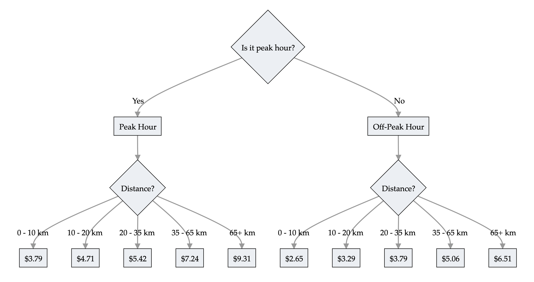
Train prices
Trees are interpretable?
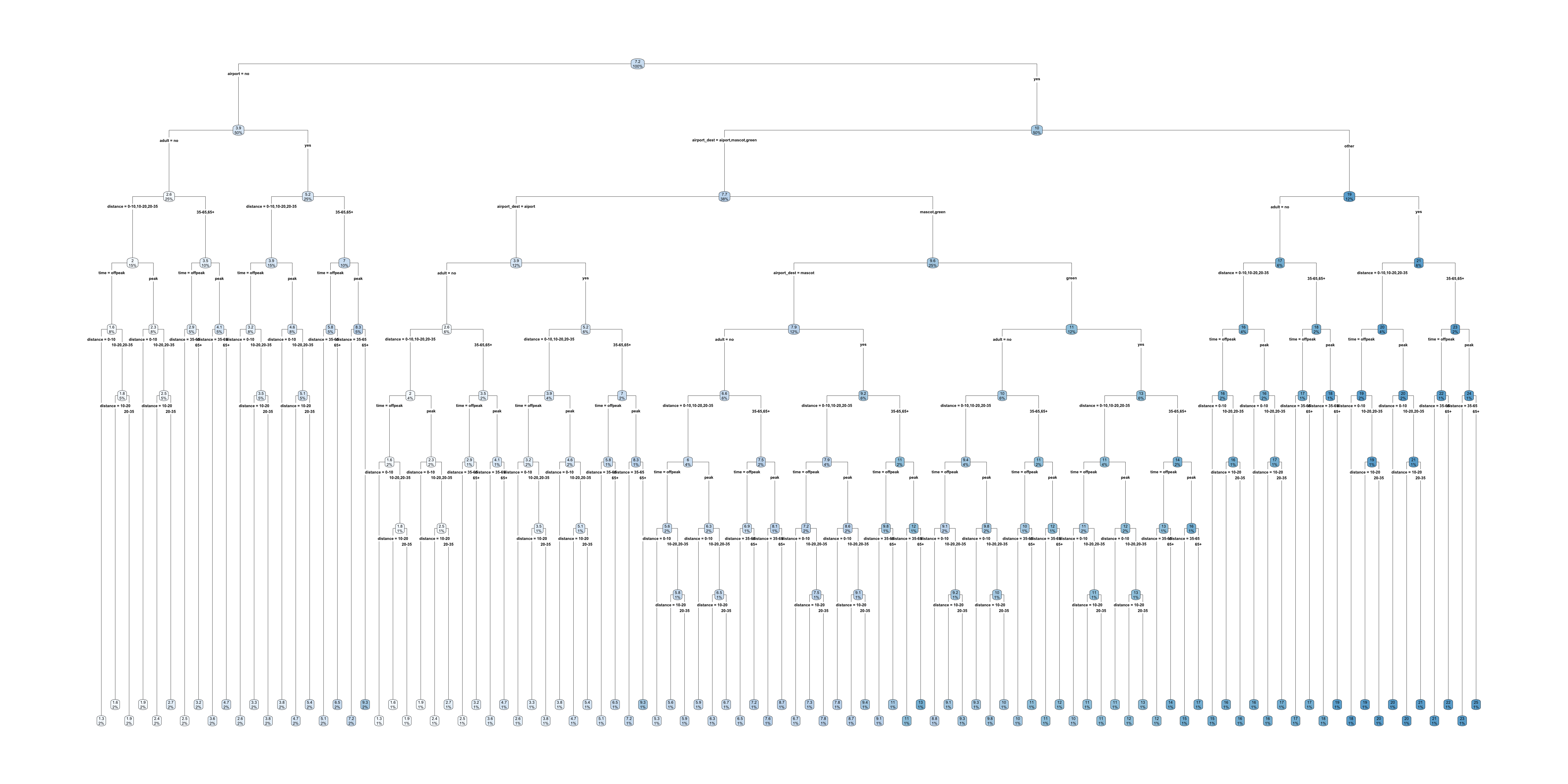
Full train pricing
Linear models
A GLM has the form
\hat{y} = g^{-1}\bigl( \beta_0 + \beta_1 x_1 + \dots + \beta_p x_p \bigr)
where \beta_0, \dots, \beta_p are the model parameters.
Global & local interpretations are easy to obtain.
LocalGLMNet
Imagine: \hat{y_i} = g^{-1}\bigl( \beta_0(\boldsymbol{x}_i) + \beta_1(\boldsymbol{x}_i) x_{i1} + \dots + \beta_p(\boldsymbol{x}_i) x_{ip} \bigr)
A GLM with local parameters \beta_0(\boldsymbol{x}_i), \dots, \beta_p(\boldsymbol{x}_i) for each observation \boldsymbol{x}_i.
The local parameters are the output of a neural network.
Post-hoc Interpretability
Lecture Outline
Interpretability
Inherent Interpretability
Post-hoc Interpretability
Explaining Specific Models
Permutation importance
Inputs: fitted model m, tabular dataset D.
Compute the reference score s of the model m on data D (for instance the accuracy for a classifier or the R^2 for a regressor).
For each feature j (column of D):
For each repetition k in {1, \dots, K}:
- Randomly shuffle column j of dataset D to generate a corrupted version of the data named \tilde{D}_{k,j}.
- Compute the score s_{k,j} of model m on corrupted data \tilde{D}_{k,j}.
Compute importance i_j for feature f_j defined as:
i_j = s - \frac{1}{K} \sum_{k=1}^{K} s_{k,j}
Source: scikit-learn documentation, permutation_importance function.
Permutation importance
LIME
Local Interpretable Model-agnostic Explanations employs an interpretable surrogate model to explain locally how the black-box model makes predictions for individual instances.
E.g. a black-box model predicts Bob’s premium as the highest among all policyholders. LIME uses an interpretable model (a linear regression) to explain how Bob’s features influence the black-box model’s prediction.
Globally vs. Locally Faithful
- Globally Faithful
-
The interpretable model’s explanations accurately reflect the behaviour of the black-box model across the entire input space.
- Locally Faithful
-
The interpretable model’s explanations accurately reflect the behaviour of the black-box model for a specific instance.
LIME aims to construct an interpretable model that mimics the black-box model’s behaviour in a locally faithful manner.
LIME Algorithm
Suppose we want to explain the instance \boldsymbol{x}_{\text{Bob}}=(1, 2, 0.5).
- Generate perturbed examples of \boldsymbol{x}_{\text{Bob}} and use the trained gamma MDN f to make predictions: \begin{align*} \boldsymbol{x}^{'(1)}_{\text{Bob}} &= (1.1, 1.9, 0.6), \quad f\big(\boldsymbol{x}^{'(1)}_{\text{Bob}}\big)=34000 \\ \boldsymbol{x}^{'(2)}_{\text{Bob}} &= (0.8, 2.1, 0.4), \quad f\big(\boldsymbol{x}^{'(2)}_{\text{Bob}}\big)=31000 \\ &\vdots \quad \quad \quad \quad\quad \quad\quad \quad\quad \quad \quad \vdots \end{align*} We can then construct a dataset of N_{\text{Examples}} perturbed examples: \mathcal{D}_{\text{LIME}} = \big(\big\{\boldsymbol{x}^{'(i)}_{\text{Bob}},f\big(\boldsymbol{x}^{'(i)}_{\text{Bob}}\big)\big\}\big)_{i=0}^{N_{\text{Examples}}}.
LIME Algorithm
- Fit an interpretable model g, i.e., a linear regression using \mathcal{D}_{\text{LIME}} and the following loss function: \mathcal{L}_{\text{LIME}}(f,g,\pi_{\boldsymbol{x}_{\text{Bob}}})=\sum_{i=1}^{N_{\text{Examples}}}\pi_{\boldsymbol{x}_{\text{Bob}}}\big(\boldsymbol{x}^{'(i)}_{\text{Bob}}\big)\cdot \bigg(f\big(\boldsymbol{x}^{'(i)}_{\text{Bob}}\big)-g\big(\boldsymbol{x}^{'(i)}_{\text{Bob}}\big)\bigg)^2, where \pi_{\boldsymbol{x}_{\text{Bob}}}\big(\boldsymbol{x}^{'(i)}_{\text{Bob}}\big) represents the distance from the perturbed example \boldsymbol{x}^{'(i)}_{\text{Bob}} to the instance to be explained \boldsymbol{x}_{\text{Bob}}.
“Explaining” to Bob
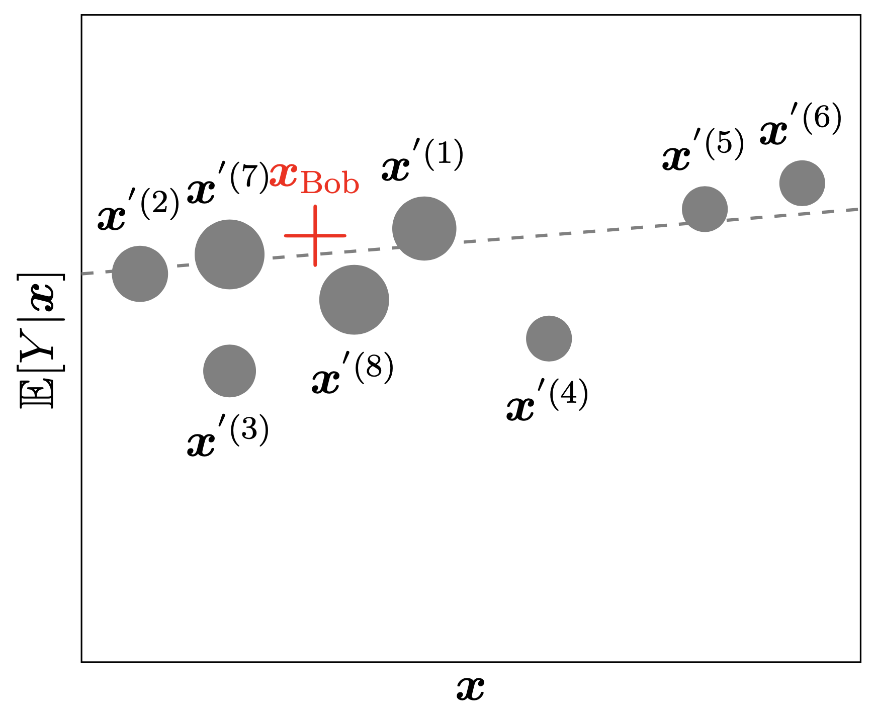
The bold red cross is the instance being explained. LIME samples instances (grey nodes), gets predictions using f (gamma MDN) and weighs them by the proximity to the instance being explained (represented here by size). The dashed line g is the learned local explanation.
SHAP Values
The SHapley Additive exPlanations (SHAP) value helps to quantify the contribution of each feature to the prediction for a specific instance.
The SHAP value for the jth feature is defined as \begin{align*} \text{SHAP}^{(j)}(\boldsymbol{x}) &= \sum_{U\subset \{1, ..., p\} \backslash \{j\}} \frac{1}{p} \binom{p-1}{|U|}^{-1} \big(\mathbb{E}[Y| \boldsymbol{x}^{(U\cup \{j\})}] - \mathbb{E}[Y|\boldsymbol{x}^{(U)}]\big), \end{align*} where p is the number of features. A positive SHAP value indicates that the variable increases the prediction value.
Reference: Lundberg & Lee (2017), A Unified Approach to Interpreting Model Predictions, Advances in Neural Information Processing Systems, 30.
Explaining Specific Models
Lecture Outline
Interpretability
Inherent Interpretability
Post-hoc Interpretability
Explaining Specific Models
Grad-CAM

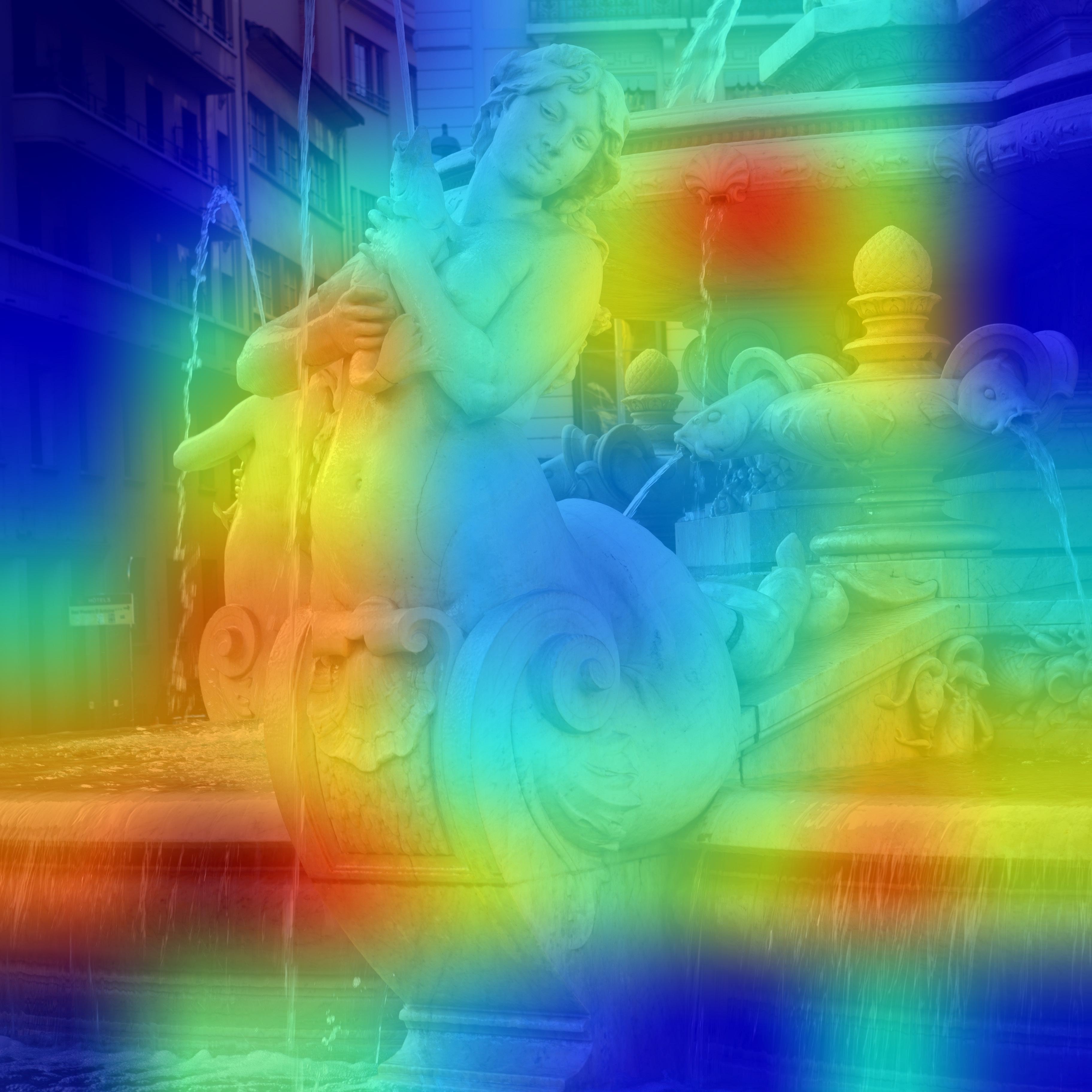
Cf. Chollet (2021), Deep Learning with Python, Section 9.4.3.
Package Versions
from watermark import watermark
print(watermark(python=True, packages="keras,matplotlib,numpy,pandas,seaborn,scipy,torch,tensorflow,tf_keras"))
Python implementation: CPython
Python version : 3.11.9
IPython version : 8.24.0
keras : 3.3.3
matplotlib: 3.8.4
numpy : 1.26.4
pandas : 2.2.2
seaborn : 0.13.2
scipy : 1.11.0
torch : 2.0.1
tensorflow: 2.16.1
tf_keras : 2.16.0
Glossary
- global interpretability
- Grad-CAM
- inherent interpretability
- LIME
- local interpretability
- permutation importance
- post-hoc interpretability
- SHAP values
![]()