Exercise: French Motor Claim Frequency

ACTL3143 & ACTL5111 Deep Learning for Actuaries

Your task is to predict the frequency distribution of car insurance claims in France.

DALL-E’s rendition of this French motor claim frequency prediction task.

French motor dataset

Show the package imports
import random
from pathlib import Path

import matplotlib.pyplot as plt
import numpy as np
import pandas as pd

import keras
from keras.callbacks import EarlyStopping
from keras.models import Sequential
from keras.layers import Dense

from sklearn.compose import make_column_transformer
from sklearn.datasets import fetch_openml
from sklearn.linear_model import LinearRegression
from sklearn.model_selection import train_test_split
from sklearn.preprocessing import OneHotEncoder, OrdinalEncoder, StandardScaler
from sklearn import set_config

import statsmodels.api as sm

set_config(transform_output="pandas")
2024-07-14 12:36:34.009101: I tensorflow/core/util/port.cc:113] oneDNN custom operations are on. You may see slightly different numerical results due to floating-point round-off errors from different computation orders. To turn them off, set the environment variable `TF_ENABLE_ONEDNN_OPTS=0`.
2024-07-14 12:36:34.110870: I tensorflow/core/platform/cpu_feature_guard.cc:210] This TensorFlow binary is optimized to use available CPU instructions in performance-critical operations.
To enable the following instructions: AVX2 AVX_VNNI FMA, in other operations, rebuild TensorFlow with the appropriate compiler flags.
2024-07-14 12:36:35.253023: W tensorflow/compiler/tf2tensorrt/utils/py_utils.cc:38] TF-TRT Warning: Could not find TensorRT

Download the dataset if we don’t have it already.

1if not Path("french-motor.csv").exists():
2    freq = fetch_openml(data_id=41214, as_frame=True).frame
3    freq.to_csv("french-motor.csv", index=False)
else:
4    freq = pd.read_csv("french-motor.csv")

freq
1
Checks if the dataset does not already exist within the Jupyter Notebook directory.
2
Fetches the dataset from OpenML
3
Converts the dataset into csv format
4
If it already exists, then read in the dataset from the file.
IDpol ClaimNb Exposure Area VehPower VehAge DrivAge BonusMalus VehBrand VehGas Density Region
0 1.0 1 0.10000 D 5 0 55 50 B12 'Regular' 1217 R82
1 3.0 1 0.77000 D 5 0 55 50 B12 'Regular' 1217 R82
2 5.0 1 0.75000 B 6 2 52 50 B12 'Diesel' 54 R22
3 10.0 1 0.09000 B 7 0 46 50 B12 'Diesel' 76 R72
4 11.0 1 0.84000 B 7 0 46 50 B12 'Diesel' 76 R72
... ... ... ... ... ... ... ... ... ... ... ... ...
678008 6114326.0 0 0.00274 E 4 0 54 50 B12 'Regular' 3317 R93
678009 6114327.0 0 0.00274 E 4 0 41 95 B12 'Regular' 9850 R11
678010 6114328.0 0 0.00274 D 6 2 45 50 B12 'Diesel' 1323 R82
678011 6114329.0 0 0.00274 B 4 0 60 50 B12 'Regular' 95 R26
678012 6114330.0 0 0.00274 B 7 6 29 54 B12 'Diesel' 65 R72

678013 rows × 12 columns

Data dictionary

  • IDpol: policy number (unique identifier)
  • Area: area code (categorical, ordinal)
  • BonusMalus: bonus-malus level between 50 and 230 (with reference level 100)
  • Density: density of inhabitants per km2 in the city of the living place of the driver
  • DrivAge: age of the (most common) driver in years
  • Exposure: total exposure in yearly units
  • Region: regions in France (prior to 2016)
  • VehAge: age of the car in years
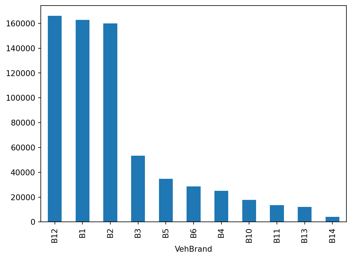
  • VehBrand: car brand (categorical, nominal)
  • VehGas: diesel or regular fuel car (binary)
  • VehPower: power of the car (categorical, ordinal)
  • ClaimNb: number of claims on the given policy (target variable)
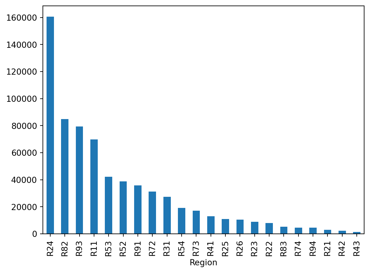
Region column

French Administrative Regions

Poisson regression

The model

Have \{ (\boldsymbol{x}_i, y_i) \}_{i=1, \dots, n} for \boldsymbol{x}_i \in \mathbb{R}^{47} and y_i \in \mathbb{N}_0.

Assume the distribution Y_i \sim \mathsf{Poisson}(\lambda(\boldsymbol{x}_i))

We have \mathbb{E} Y_i = \lambda(\boldsymbol{x}_i). The NN takes \boldsymbol{x}_i & predicts \mathbb{E} Y_i.

Note

For insurance, this is a bit weird. The exposures are different for each policy.

\lambda(\boldsymbol{x}_i) is the expected number of claims for the duration of policy i’s contract.

Normally, \text{Exposure}_i \not\in \boldsymbol{x}_i, and \lambda(\boldsymbol{x}_i) is the expected rate per year, then Y_i \sim \mathsf{Poisson}(\text{Exposure}_i \times \lambda(\boldsymbol{x}_i)).

Help about the “poisson” loss

help(keras.losses.poisson)
Help on function poisson in module keras.src.losses.losses:

poisson(y_true, y_pred)
    Computes the Poisson loss between y_true and y_pred.
    
    Formula:
    
    ```python
    loss = y_pred - y_true * log(y_pred)
    ```
    
    Args:
        y_true: Ground truth values. shape = `[batch_size, d0, .. dN]`.
        y_pred: The predicted values. shape = `[batch_size, d0, .. dN]`.
    
    Returns:
        Poisson loss values with shape = `[batch_size, d0, .. dN-1]`.
    
    Example:
    
    >>> y_true = np.random.randint(0, 2, size=(2, 3))
    >>> y_pred = np.random.random(size=(2, 3))
    >>> loss = keras.losses.poisson(y_true, y_pred)
    >>> assert loss.shape == (2,)
    >>> y_pred = y_pred + 1e-7
    >>> assert np.allclose(
    ...     loss, np.mean(y_pred - y_true * np.log(y_pred), axis=-1),
    ...     atol=1e-5)

Poisson probabilities

Since the probability mass function (p.m.f.) of the N \sim \mathsf{Poisson}(\lambda) distribution is \mathbb{P}(N = k) = \frac{\lambda^k \mathrm{e}^{-\lambda}}{k!} then the p.m.f. of Y_i \sim \mathsf{Poisson}(\lambda(\boldsymbol{x}_i)) is

\mathbb{P}(Y_i = y_i) = \frac{ \lambda(\boldsymbol{x}_i)^{y_i} \, \mathrm{e}^{-\lambda(\boldsymbol{x}_i)} }{y_i!}

The likelihood of a sample is then \mathbb{P}(Y_1 = y_1, \dots, Y_n = y_n) = \prod_{i=1}^n \mathbb{P}(Y_i = y_i).

Log-likelihood

Therefore, the likelihood of \{ (\boldsymbol{x}_i, y_i) \}_{i=1, \dots, n} is

L = \prod_{i=1}^n \frac{ \lambda(\boldsymbol{x}_i)^{y_i} \, \mathrm{e}^{-\lambda(\boldsymbol{x}_i)} }{y_i!}

so the log-likelihood is

\begin{aligned} \ell &= \sum_{i=1}^n \log \bigl( \frac{ \lambda(\boldsymbol{x}_i)^{y_i} \, \mathrm{e}^{-\lambda(\boldsymbol{x}_i)} }{y_i!} \bigr) \\ &= \sum_{i=1}^n y_i \log \bigl( \lambda(\boldsymbol{x}_i) \bigr) - \lambda(\boldsymbol{x}_i) - \log(y_i!) . \end{aligned}

Maximising the likelihood

Want to find the best NN \lambda^* such that: \begin{aligned} \lambda^* &= \arg\max_{\lambda} \sum_{i=1}^n y_i \log \bigl( \lambda(\boldsymbol{x}_i) \bigr) - \lambda(\boldsymbol{x}_i) - \log(y_i!) \\ &= \arg\max_{\lambda} \sum_{i=1}^n y_i \log \bigl( \lambda(\boldsymbol{x}_i) \bigr) - \lambda(\boldsymbol{x}_i) \\ &= \arg\min_{\lambda} \sum_{i=1}^n \lambda(\boldsymbol{x}_i) - y_i \log \bigl( \lambda(\boldsymbol{x}_i)\bigr) \\ &= \arg\min_{\lambda} \frac{1}{n} \sum_{i=1}^n \lambda(\boldsymbol{x}_i) - y_i \log \bigl( \lambda(\boldsymbol{x}_i)\bigr) . \end{aligned}

Keras’ “poisson” loss again

help(poisson)
Help on function poisson in module keras.losses:

poisson(y_true, y_pred)
    Computes the Poisson loss between y_true and y_pred.
    
    The Poisson loss is the mean of the elements of the `Tensor`
    `y_pred - y_true * log(y_pred)`.
  
...

In other words, \text{PoissonLoss} = \frac{1}{n} \sum_{i=1}^n \lambda(\boldsymbol{x}_i) - y_i \log \bigl( \lambda(\boldsymbol{x}_i) \bigr) .

Poisson deviance

D = 2 \sum_{i=1}^n y_i \log\bigl( \frac{y_i}{\lambda(\boldsymbol{x}_i)} \bigr) - \bigl( y_i - \lambda(\boldsymbol{x}_i) \bigr) .

from sklearn.metrics import mean_poisson_deviance
y_true = [0, 2, 1]
y_pred = [0.1, 0.9, 0.8]
mean_poisson_deviance(y_true, y_pred)
0.4134392958331687
deviance = 0
for y_i, yhat_i in zip(y_true, y_pred):
  firstTerm = y_i * np.log(y_i / yhat_i) if y_i > 0 else 0
  deviance += 2 * (firstTerm - (y_i - yhat_i))
meanDeviance = deviance / len(y_true)
deviance, meanDeviance
(1.240317887499506, 0.4134392958331687)

Poisson deviance as a loss function

Want to find the best NN \lambda^* such that: \begin{aligned} \lambda^* &= \arg\min_{\lambda} \, 2 \sum_{i=1}^n y_i \log\bigl( \frac{y_i}{\lambda(\boldsymbol{x}_i)} \bigr) - \bigl( y_i - \lambda(\boldsymbol{x}_i) \bigr) \\ &= \arg\min_{\lambda} \sum_{i=1}^n y_i \log( y_i ) - y_i \log\bigl( \lambda(\boldsymbol{x}_i) \bigr) - y_i + \lambda(\boldsymbol{x}_i) \\ &= \arg\min_{\lambda} \sum_{i=1}^n - y_i \log\bigl( \lambda(\boldsymbol{x}_i) \bigr) + \lambda(\boldsymbol{x}_i) \\ &= \arg\min_{\lambda} \sum_{i=1}^n \lambda(\boldsymbol{x}_i) - y_i \log\bigl( \lambda(\boldsymbol{x}_i) \bigr) . \end{aligned}

GLM

Split the data

X = freq.drop(columns=["ClaimNb", "IDpol"])
y = freq["ClaimNb"]

X_main, X_test, y_main, y_test = train_test_split(X, y, test_size=0.2, random_state=42)
X_train, X_val, y_train, y_val = train_test_split(X_main, y_main, test_size=0.25, random_state=42)

TODO: Modify this to do a stratified split. That is, the distribution of ClaimNb should be (about) the same in the training, validation, and test sets.

Preprocess the inputs for a GLM

ct_glm = make_column_transformer(
  (OrdinalEncoder(), ["Area"]),
1  (OneHotEncoder(sparse_output=False, drop="first"),
      ["VehGas", "VehBrand", "Region"]),
  remainder="passthrough",
  verbose_feature_names_out=False
)
2X_train_glm = sm.add_constant(ct_glm.fit_transform(X_train))
X_val_glm = sm.add_constant(ct_glm.transform(X_val))
X_test_glm = sm.add_constant(ct_glm.transform(X_test))

X_train_glm
1
The drop="first" parameter is used to avoid multicollinearity in the model.
2
The sm.add_constant function adds a column of ones to the input matrix.
const Area VehGas_'Regular' VehBrand_B10 VehBrand_B11 VehBrand_B12 VehBrand_B13 VehBrand_B14 VehBrand_B2 VehBrand_B3 ... Region_R83 Region_R91 Region_R93 Region_R94 Exposure VehPower VehAge DrivAge BonusMalus Density
642604 1.0 3.0 0.0 0.0 0.0 1.0 0.0 0.0 0.0 0.0 ... 0.0 1.0 0.0 0.0 0.74 11 1 50 50 824
394020 1.0 0.0 0.0 0.0 0.0 0.0 0.0 0.0 1.0 0.0 ... 0.0 0.0 0.0 0.0 1.00 6 10 51 55 42
104966 1.0 3.0 1.0 0.0 0.0 0.0 0.0 0.0 1.0 0.0 ... 0.0 0.0 0.0 0.0 1.00 4 20 81 50 747
438856 1.0 0.0 0.0 0.0 0.0 1.0 0.0 0.0 0.0 0.0 ... 0.0 0.0 0.0 0.0 0.25 7 3 44 50 23
87109 1.0 3.0 1.0 0.0 0.0 1.0 0.0 0.0 0.0 0.0 ... 0.0 0.0 1.0 0.0 0.12 7 1 52 50 721
... ... ... ... ... ... ... ... ... ... ... ... ... ... ... ... ... ... ... ... ... ...
99179 1.0 2.0 1.0 0.0 0.0 0.0 0.0 0.0 0.0 0.0 ... 0.0 0.0 0.0 0.0 0.31 7 6 49 50 119
523093 1.0 4.0 0.0 0.0 0.0 1.0 0.0 0.0 0.0 0.0 ... 0.0 0.0 1.0 0.0 0.04 7 0 43 51 4762
143052 1.0 2.0 0.0 0.0 0.0 0.0 1.0 0.0 0.0 0.0 ... 0.0 0.0 0.0 0.0 1.00 6 6 36 50 133
606805 1.0 1.0 0.0 0.0 0.0 1.0 0.0 0.0 0.0 0.0 ... 0.0 0.0 0.0 0.0 0.48 5 0 73 50 79
228897 1.0 0.0 1.0 0.0 0.0 0.0 0.0 0.0 0.0 1.0 ... 0.0 0.0 1.0 0.0 1.00 4 5 76 50 34

406807 rows × 40 columns

Alternatively, you can try to reproduce this using the patsy library and an R-style formula.

Fit a GLM

Using the statsmodels package, we can fit a Poisson regression model.

glm = sm.GLM(y_train, X_train_glm, family=sm.families.Poisson())
glm_results = glm.fit()
glm_results.summary()
Generalized Linear Model Regression Results
Dep. Variable: ClaimNb No. Observations: 406807
Model: GLM Df Residuals: 406767
Model Family: Poisson Df Model: 39
Link Function: Log Scale: 1.0000
Method: IRLS Log-Likelihood: -83303.
Date: Sun, 14 Jul 2024 Deviance: 1.2522e+05
Time: 12:36:48 Pearson chi2: 4.56e+05
No. Iterations: 7 Pseudo R-squ. (CS): 0.01256
Covariance Type: nonrobust
coef std err z P>|z| [0.025 0.975]
const -5.2621 0.061 -86.094 0.000 -5.382 -5.142
Area 0.0529 0.007 7.852 0.000 0.040 0.066
VehGas_'Regular' 0.0779 0.014 5.497 0.000 0.050 0.106
VehBrand_B10 -0.0629 0.049 -1.296 0.195 -0.158 0.032
VehBrand_B11 -0.0238 0.053 -0.450 0.653 -0.128 0.080
VehBrand_B12 0.0577 0.023 2.528 0.011 0.013 0.103
VehBrand_B13 0.0137 0.053 0.257 0.797 -0.091 0.118
VehBrand_B14 -0.2025 0.104 -1.943 0.052 -0.407 0.002
VehBrand_B2 -0.0017 0.020 -0.085 0.932 -0.040 0.037
VehBrand_B3 -0.0357 0.029 -1.250 0.211 -0.092 0.020
VehBrand_B4 -0.0373 0.039 -0.968 0.333 -0.113 0.038
VehBrand_B5 0.0837 0.032 2.620 0.009 0.021 0.146
VehBrand_B6 -0.0441 0.036 -1.208 0.227 -0.116 0.027
Region_R21 0.0675 0.108 0.628 0.530 -0.143 0.278
Region_R22 0.0905 0.066 1.363 0.173 -0.040 0.221
Region_R23 -0.1839 0.078 -2.368 0.018 -0.336 -0.032
Region_R24 0.1573 0.032 4.975 0.000 0.095 0.219
Region_R25 0.0126 0.060 0.210 0.833 -0.105 0.130
Region_R26 -0.0466 0.064 -0.725 0.469 -0.173 0.079
Region_R31 -0.0591 0.044 -1.332 0.183 -0.146 0.028
Region_R41 -0.2423 0.061 -3.997 0.000 -0.361 -0.123
Region_R42 0.0151 0.118 0.128 0.898 -0.216 0.247
Region_R43 -0.0340 0.171 -0.199 0.842 -0.369 0.301
Region_R52 0.0445 0.039 1.136 0.256 -0.032 0.121
Region_R53 0.1868 0.037 5.031 0.000 0.114 0.260
Region_R54 0.0046 0.050 0.091 0.927 -0.094 0.103
Region_R72 -0.1490 0.044 -3.364 0.001 -0.236 -0.062
Region_R73 -0.1302 0.055 -2.358 0.018 -0.238 -0.022
Region_R74 0.2443 0.084 2.901 0.004 0.079 0.409
Region_R82 0.1525 0.031 4.972 0.000 0.092 0.213
Region_R83 -0.2533 0.096 -2.627 0.009 -0.442 -0.064
Region_R91 -0.0782 0.042 -1.849 0.064 -0.161 0.005
Region_R93 0.0007 0.032 0.022 0.983 -0.063 0.064
Region_R94 0.1519 0.085 1.790 0.074 -0.014 0.318
Exposure 1.0462 0.021 49.448 0.000 1.005 1.088
VehPower 0.0097 0.004 2.733 0.006 0.003 0.017
VehAge -0.0350 0.001 -23.398 0.000 -0.038 -0.032
DrivAge 0.0091 0.001 17.680 0.000 0.008 0.010
BonusMalus 0.0202 0.000 49.319 0.000 0.019 0.021
Density -8.998e-07 2.22e-06 -0.406 0.685 -5.25e-06 3.45e-06

Extract the Poisson deviance from the GLM

glm_results.deviance
125222.6772692274

Mean Poisson deviance:

glm_results.deviance / len(y_train)
0.30781839365897684

Using the mean_poisson_deviance function:

mean_poisson_deviance(y_train, glm_results.predict(X_train_glm))
0.30781839365897684

Validation set mean Poisson deviance:

mean_poisson_deviance(y_val, glm_results.predict(X_val_glm))
0.3091974082275962

TODO: Add in lasso or ridge regularization to the GLM using the validation set.

Neural network

Look at the counts of the Region and VehBrand columns

freq["Region"].value_counts().plot(kind="bar")

freq["VehBrand"].value_counts().plot(kind="bar")

TODO: Consider combining the least frequent categories into a single category. That would reduce the cardinality of the categorical columns, and hence the number of input features.

Prepare the data for a neural network

ct = make_column_transformer(
  (OrdinalEncoder(), ["Area"]),
1  (OneHotEncoder(sparse_output=False, drop="if_binary"),
      ["VehGas", "VehBrand", "Region"]),
  remainder=StandardScaler(),
  verbose_feature_names_out=False
)
X_train_ct = ct.fit_transform(X_train)
X_val_ct = ct.transform(X_val)
X_test_ct = ct.transform(X_test)

X_train_ct
1
The drop="if_binary" parameter will only drop the first column if the column is binary (i.e. for the VehGas column).
Area VehGas_'Regular' VehBrand_B1 VehBrand_B10 VehBrand_B11 VehBrand_B12 VehBrand_B13 VehBrand_B14 VehBrand_B2 VehBrand_B3 ... Region_R83 Region_R91 Region_R93 Region_R94 Exposure VehPower VehAge DrivAge BonusMalus Density
642604 3.0 0.0 0.0 0.0 0.0 1.0 0.0 0.0 0.0 0.0 ... 0.0 1.0 0.0 0.0 0.579995 2.216304 -1.068169 0.319694 -0.623906 -0.244407
394020 0.0 0.0 0.0 0.0 0.0 0.0 0.0 0.0 1.0 0.0 ... 0.0 0.0 0.0 0.0 1.293590 -0.221879 0.522740 0.390412 -0.304423 -0.441611
104966 3.0 1.0 0.0 0.0 0.0 0.0 0.0 0.0 1.0 0.0 ... 0.0 0.0 0.0 0.0 1.293590 -1.197153 2.290416 2.511980 -0.623906 -0.263825
438856 0.0 0.0 0.0 0.0 0.0 1.0 0.0 0.0 0.0 0.0 ... 0.0 0.0 0.0 0.0 -0.764858 0.265757 -0.714634 -0.104620 -0.623906 -0.446403
87109 3.0 1.0 0.0 0.0 0.0 1.0 0.0 0.0 0.0 0.0 ... 0.0 0.0 1.0 0.0 -1.121655 0.265757 -1.068169 0.461131 -0.623906 -0.270382
... ... ... ... ... ... ... ... ... ... ... ... ... ... ... ... ... ... ... ... ... ...
99179 2.0 1.0 1.0 0.0 0.0 0.0 0.0 0.0 0.0 0.0 ... 0.0 0.0 0.0 0.0 -0.600182 0.265757 -0.184331 0.248975 -0.623906 -0.422194
523093 4.0 0.0 0.0 0.0 0.0 1.0 0.0 0.0 0.0 0.0 ... 0.0 0.0 1.0 0.0 -1.341223 0.265757 -1.244937 -0.175339 -0.560009 0.748673
143052 2.0 0.0 0.0 0.0 0.0 0.0 1.0 0.0 0.0 0.0 ... 0.0 0.0 0.0 0.0 1.293590 -0.221879 -0.184331 -0.670371 -0.623906 -0.418663
606805 1.0 0.0 0.0 0.0 0.0 1.0 0.0 0.0 0.0 0.0 ... 0.0 0.0 0.0 0.0 -0.133600 -0.709516 -1.244937 1.946228 -0.623906 -0.432281
228897 0.0 1.0 0.0 0.0 0.0 0.0 0.0 0.0 0.0 1.0 ... 0.0 0.0 1.0 0.0 1.293590 -1.197153 -0.361099 2.158385 -0.623906 -0.443629

406807 rows × 41 columns

Fit a neural network

model = Sequential([
    Dense(64, activation='leaky_relu', input_shape=(X_train_ct.shape[1],)),
    Dense(32, activation='leaky_relu'),
    Dense(1, activation='exponential')
])

model.compile(optimizer='adam', loss='poisson')
es = EarlyStopping(patience=5, restore_best_weights=True)
history = model.fit(X_train_ct, y_train, validation_data=(X_val_ct, y_val), epochs=100, callbacks=[es], verbose=0)

Evaluate

model.evaluate(X_train_ct, y_train, verbose=0)
0.19423706829547882
y_train_pred = model.predict(X_train_ct, verbose=0)
mean_poisson_deviance(y_train, y_train_pred)
0.29141035666769616
y_val_pred = model.predict(X_val_ct, verbose=0)
mean_poisson_deviance(y_val, y_val_pred)
0.297274932858001

TODO: Change exposure to be an offset in the Poisson regression model, both in the GLM and the neural network.