def permutation_test(model, X, y, num_reps=1, seed=42):
    """
    Run the permutation test for variable importance.
    Returns matrix of shape (X.shape[1], len(model.evaluate(X, y))).
    """
    rnd.seed(seed)
    scores = []

    for j in range(X.shape[1]):
        original_column = np.copy(X[:, j])
        col_scores = []

        for r in range(num_reps):
            rnd.shuffle(X[:,j])
            col_scores.append(model.evaluate(X, y, verbose=0))

        scores.append(np.mean(col_scores, axis=0))
        X[:,j] = original_column

return np.array(scores)Interpretability
ACTL3143 & ACTL5111 Deep Learning for Actuaries
Patrick Laub
Interpretability
Lecture Outline
Interpretability
Inherent Interpretability
Post-hoc Interpretability
Illustrative Example
Illustrative Example (Fixed)
Interpretability
- Interpretability Definition
-
Interpretability refers to the ease with which one can understand and comprehend the model’s algorithm and predictions.
Interpretability of black-box models can be crucial to ascertaining trust.
Interpretability is about transparency, about understanding exactly why and how the model is generating predictions, and therefore, it is important to observe the inner mechanics of the algorithm considered. This leads to interpreting the model’s parameters and features used to determine the given output. Explainability is about explaining the behavior of the model in human terms.
Source: Charpentier (2024), Insurance, Biases, Discrimination and Fairness, Springer.
Husky vs. Wolf
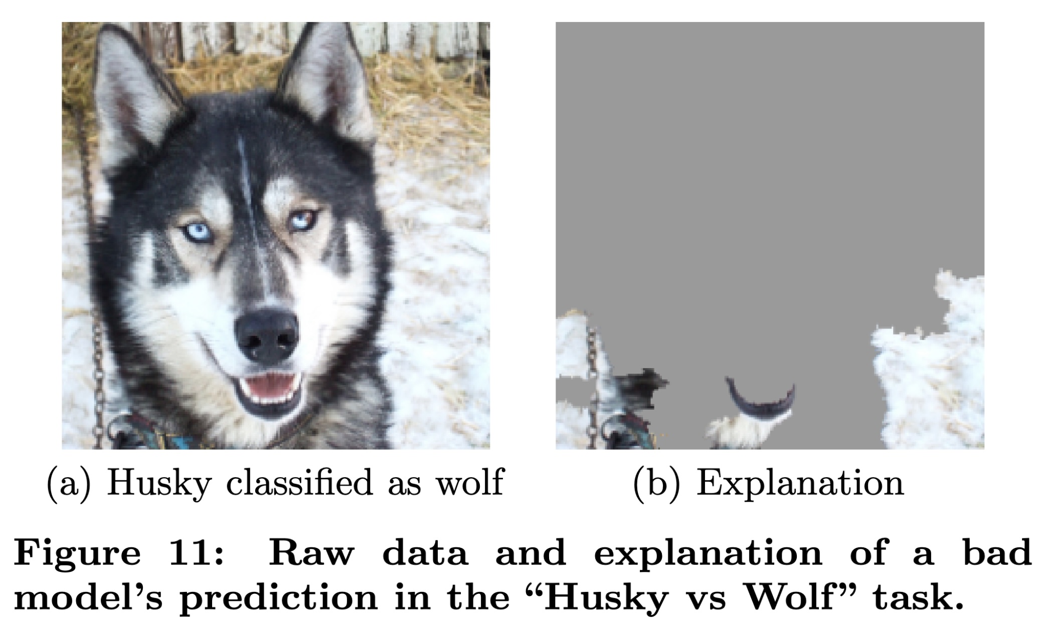
A well-known anecdote in the explainability literature.
Ribeiro et al. (2016), “Why should I trust you?” Explaining the predictions of any classifier, 22nd ACM SIGKDD conference.
Aspects of Interpretability
- Inherent Interpretability
-
The model is interpretable by design.
- Post-hoc Interpretability
-
The model is not interpretable by design, but we can use other methods to explain the model.
- Global Interpretability
-
The ability to understand how the model works.
- Local Interpretability
-
The ability to interpret/understand each prediction.
Inherent Interpretability
Lecture Outline
Interpretability
Inherent Interpretability
Post-hoc Interpretability
Illustrative Example
Illustrative Example (Fixed)

Rudin (2019), Stop explaining black box machine learning models for high stakes decisions and use interpretable models instead, Nature Machine Intelligence.
Trees are interpretable!
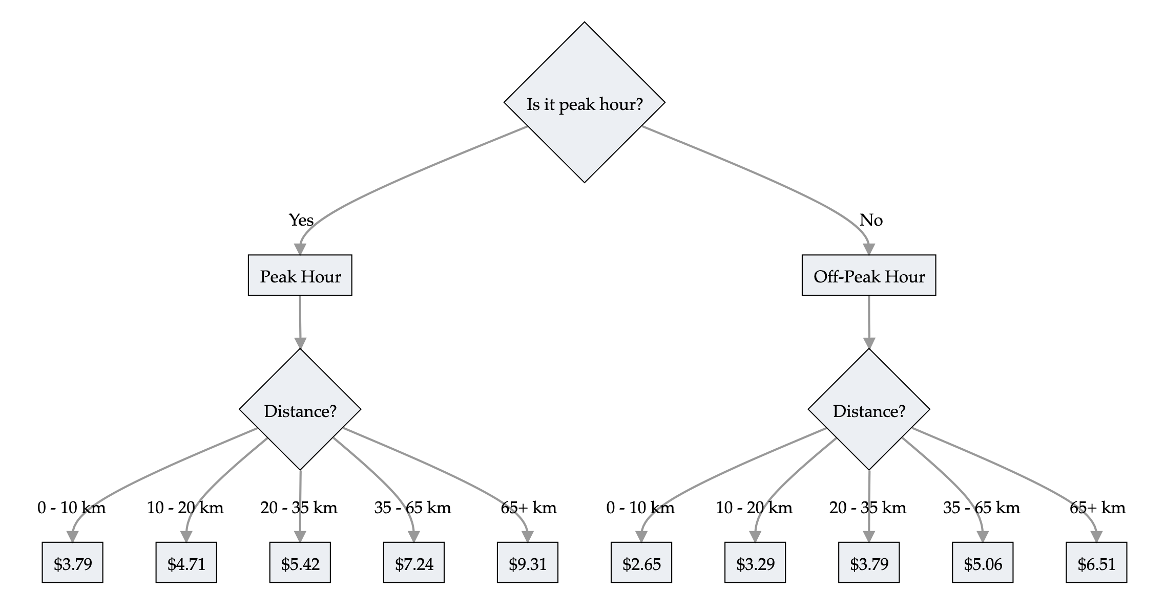
Train prices
Trees are interpretable?
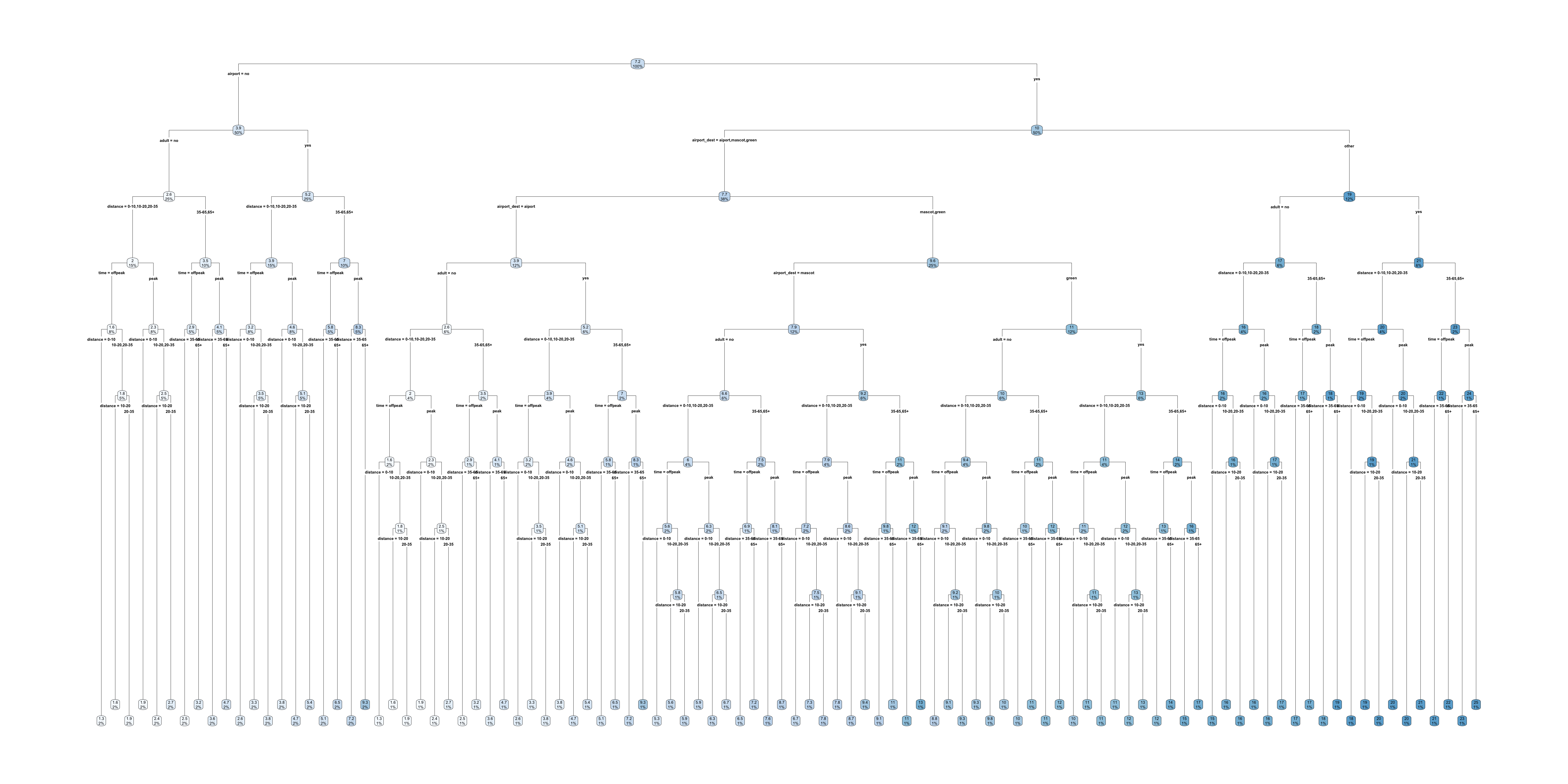
Full train pricing
Linear models & LocalGLMNet
A GLM has the form
\hat{y} = g^{-1}\bigl( \beta_0 + \beta_1 x_1 + \dots + \beta_p x_p \bigr)
where \beta_0, \dots, \beta_p are the model parameters.
Global & local interpretations are easy to obtain.
LocalGLMNet extends this to a neural network.
\hat{y_i} = g^{-1}\bigl( \beta_0(\boldsymbol{x}_i) + \beta_1(\boldsymbol{x}_i) x_{i1} + \dots + \beta_p(\boldsymbol{x}_i) x_{ip} \bigr)
A GLM with local parameters \beta_0(\boldsymbol{x}_i), \dots, \beta_p(\boldsymbol{x}_i) for each observation \boldsymbol{x}_i. The local parameters are the output of a neural network.
Source: Richman and Wüthrich (2023), LocalGLMnet: interpretable deep learning for tabular data, Scandinavian Actuarial Journal (2023.1), pp. 71-95.
Post-hoc Interpretability
Lecture Outline
Interpretability
Inherent Interpretability
Post-hoc Interpretability
Illustrative Example
Illustrative Example (Fixed)
Permutation importance
Inputs: fitted model m, tabular dataset D.
Compute the reference score s of the model m on data D (for instance the accuracy for a classifier or the R^2 for a regressor).
For each feature j (column of D):
For each repetition k in {1, \dots, K}:
- Randomly shuffle column j of dataset D to generate a corrupted version of the data named \tilde{D}_{k,j}.
- Compute the score s_{k,j} of model m on corrupted data \tilde{D}_{k,j}.
Compute importance i_j for feature f_j defined as:
i_j = s - \frac{1}{K} \sum_{k=1}^{K} s_{k,j}
Originally proposed by Breiman (2001), Random forests, Machine learning (45), pp. 5-32.
Extended by Fisher et al. (2019), All models are wrong, but many are useful: Learning a variable’s importance by studying an entire class of prediction models simultaneously, Journal of Machine Learning Research (20.177), pp. 1-81.
Source: scikit-learn documentation, permutation_importance function.
Permutation importance
LIME
Local Interpretable Model-agnostic Explanations employs an interpretable surrogate model to explain locally how the black-box model makes predictions for individual instances.
E.g. a black-box model predicts Bob’s premium as the highest among all policyholders. LIME uses an interpretable model (a linear regression) to explain how Bob’s features influence the black-box model’s prediction.
Globally vs. Locally Faithful
- Globally Faithful
-
The interpretable model’s explanations accurately reflect the behaviour of the black-box model across the entire input space.
- Locally Faithful
-
The interpretable model’s explanations accurately reflect the behaviour of the black-box model for a specific instance.
LIME aims to construct an interpretable model that mimics the black-box model’s behaviour in a locally faithful manner.
LIME Algorithm
Suppose we want to explain the instance \boldsymbol{x}_{\text{Bob}}=(1, 2, 0.5).
- Generate perturbed examples of \boldsymbol{x}_{\text{Bob}} and use the trained gamma MDN f to make predictions: \begin{align*} \boldsymbol{x}^{'(1)}_{\text{Bob}} &= (1.1, 1.9, 0.6), \quad f\big(\boldsymbol{x}^{'(1)}_{\text{Bob}}\big)=34000 \\ \boldsymbol{x}^{'(2)}_{\text{Bob}} &= (0.8, 2.1, 0.4), \quad f\big(\boldsymbol{x}^{'(2)}_{\text{Bob}}\big)=31000 \\ &\vdots \quad \quad \quad \quad\quad \quad\quad \quad\quad \quad \quad \vdots \end{align*} We can then construct a dataset of N_{\text{Examples}} perturbed examples: \mathcal{D}_{\text{LIME}} = \big(\big\{\boldsymbol{x}^{'(i)}_{\text{Bob}},f\big(\boldsymbol{x}^{'(i)}_{\text{Bob}}\big)\big\}\big)_{i=0}^{N_{\text{Examples}}}.
LIME Algorithm
- Fit an interpretable model g, i.e., a linear regression using \mathcal{D}_{\text{LIME}} and the following loss function: \mathcal{L}_{\text{LIME}}(f,g,\pi_{\boldsymbol{x}_{\text{Bob}}})=\sum_{i=1}^{N_{\text{Examples}}}\pi_{\boldsymbol{x}_{\text{Bob}}}\big(\boldsymbol{x}^{'(i)}_{\text{Bob}}\big)\cdot \bigg(f\big(\boldsymbol{x}^{'(i)}_{\text{Bob}}\big)-g\big(\boldsymbol{x}^{'(i)}_{\text{Bob}}\big)\bigg)^2, where \pi_{\boldsymbol{x}_{\text{Bob}}}\big(\boldsymbol{x}^{'(i)}_{\text{Bob}}\big) represents the distance from the perturbed example \boldsymbol{x}^{'(i)}_{\text{Bob}} to the instance to be explained \boldsymbol{x}_{\text{Bob}}.
“Explaining” to Bob
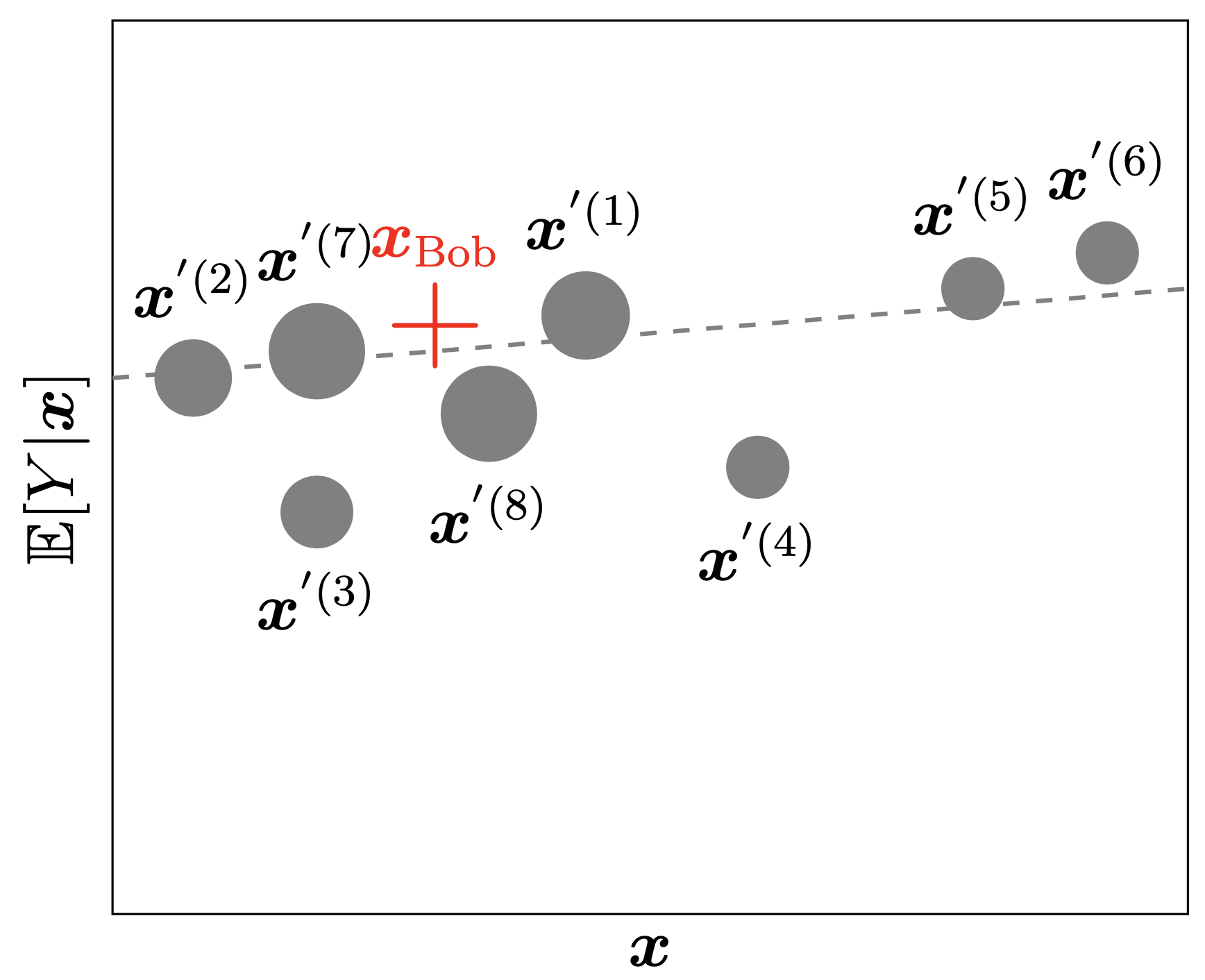
The bold red cross is the instance being explained. LIME samples instances (grey nodes), gets predictions using f (gamma MDN) and weighs them by the proximity to the instance being explained (represented here by size). The dashed line g is the learned local explanation.
SHAP Values
The SHapley Additive exPlanations (SHAP) value helps to quantify the contribution of each feature to the prediction for a specific instance.
The SHAP value for the jth feature is defined as \begin{align*} \text{SHAP}^{(j)}(\boldsymbol{x}) &= \sum_{U\subset \{1, ..., p\} \backslash \{j\}} \frac{1}{p} \binom{p-1}{|U|}^{-1} \big(\mathbb{E}[Y| \boldsymbol{x}^{(U\cup \{j\})}] - \mathbb{E}[Y|\boldsymbol{x}^{(U)}]\big), \end{align*} where p is the number of features. A positive SHAP value indicates that the variable increases the prediction value.
Reference: Lundberg & Lee (2017), A Unified Approach to Interpreting Model Predictions, Advances in Neural Information Processing Systems, 30.
Grad-CAM

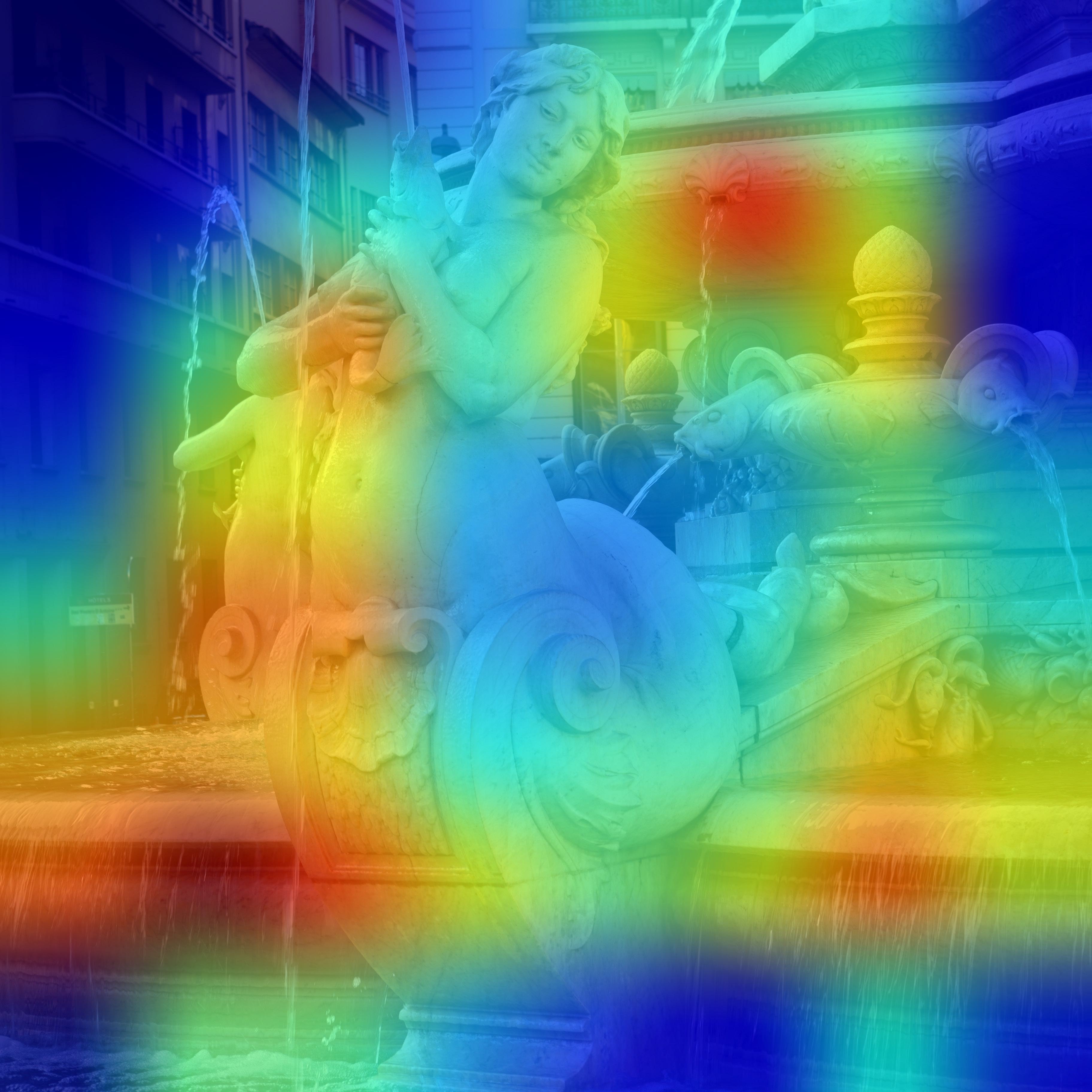
See, e.g., Keras tutorial.
See Chollet (2021), Deep Learning with Python, Section 9.4.3.
Criticism
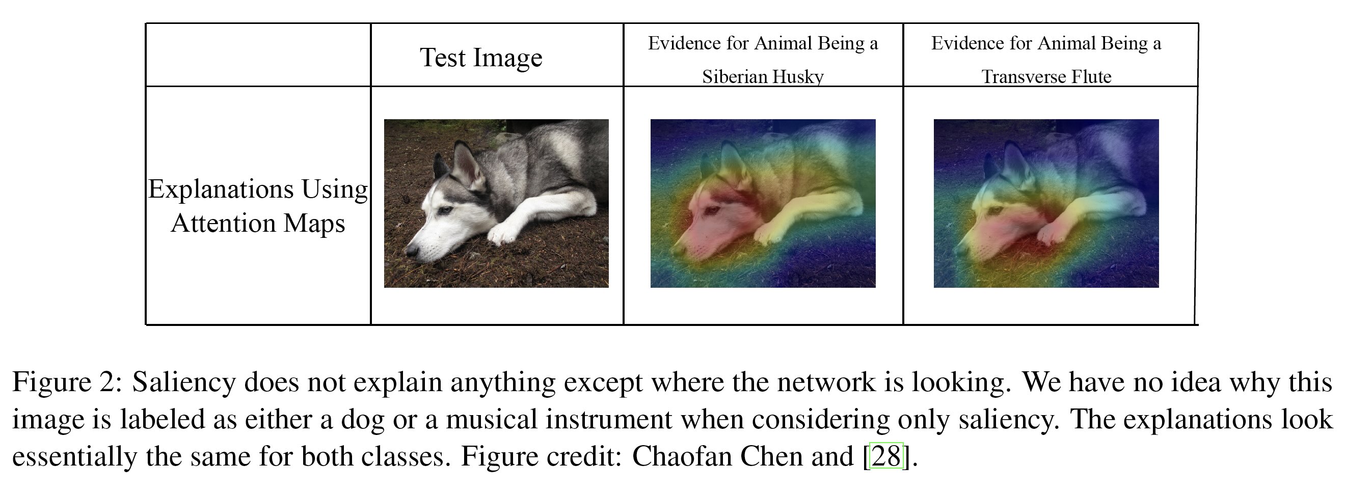
Multiple conflicting explanations.
Source: Rudin (2019), Stop explaining black box machine learning models for high stakes decisions and use interpretable models instead, Nature Machine Intelligence.
Illustrative Example
Lecture Outline
Interpretability
Inherent Interpretability
Post-hoc Interpretability
Illustrative Example
Illustrative Example (Fixed)
First attempt at NLP task
Code
df_raw = pd.read_parquet("../Natural-Language-Processing/NHTSA_NMVCCS_extract.parquet.gzip")

df_raw["NUM_VEHICLES"] = df_raw["NUMTOTV"].map(lambda x: str(x) if x <= 2 else "3+")

weather_cols = [f"WEATHER{i}" for i in range(1, 9)]
features = df_raw[["SUMMARY_EN"] + weather_cols]

target_labels = df_raw["NUM_VEHICLES"]
target = LabelEncoder().fit_transform(target_labels)

X_main, X_test, y_main, y_test = train_test_split(features, target, test_size=0.2, random_state=1)
X_train, X_val, y_train, y_val = train_test_split(X_main, y_main, test_size=0.25, random_state=1)0 V1, a 2000 Pontiac Montana minivan, made a lef...
1 The crash occurred in the eastbound lane of a ...
2 This crash occurred just after the noon time h...
...
6946 The crash occurred in the eastbound lanes of a...
6947 This single-vehicle crash occurred in a rural ...
6948 This two vehicle daytime collision occurred mi...
Name: SUMMARY_EN, Length: 6949, dtype: objectSource: JSchelldorfer’s GitHub.
Bag of words for the top 1,000 words
Code
def vectorise_dataset(X, vect, txt_col="SUMMARY_EN", dataframe=False):
    X_vects = vect.transform(X[txt_col]).toarray()
    X_other = X.drop(txt_col, axis=1)

    if not dataframe:
        return np.concatenate([X_vects, X_other], axis=1)
    else:
        # Add column names and indices to the combined dataframe.
        vocab = list(vect.get_feature_names_out())
        X_vects_df = pd.DataFrame(X_vects, columns=vocab, index=X.index)
        return pd.concat([X_vects_df, X_other], axis=1)
vect = CountVectorizer(max_features=1_000, stop_words="english")
vect.fit(X_train["SUMMARY_EN"])
X_train_bow = vectorise_dataset(X_train, vect)
X_val_bow = vectorise_dataset(X_val, vect)
X_test_bow = vectorise_dataset(X_test, vect)
vectorise_dataset(X_train, vect, dataframe=True).head()| 10 | 105 | 113 | 12 | 15 | 150 | 16 | 17 | 18 | 180 | ... | yield | zone | WEATHER1 | WEATHER2 | WEATHER3 | WEATHER4 | WEATHER5 | WEATHER6 | WEATHER7 | WEATHER8 | |
|---|---|---|---|---|---|---|---|---|---|---|---|---|---|---|---|---|---|---|---|---|---|
| 2532 | 0 | 0 | 0 | 0 | 0 | 0 | 0 | 0 | 0 | 0 | ... | 0 | 0 | 0 | 0 | 0 | 0 | 0 | 0 | 0 | 0 |
| 6209 | 0 | 0 | 0 | 0 | 0 | 0 | 0 | 0 | 0 | 0 | ... | 0 | 0 | 0 | 0 | 0 | 0 | 0 | 0 | 0 | 0 |
| 2561 | 1 | 0 | 1 | 0 | 0 | 0 | 0 | 0 | 0 | 0 | ... | 0 | 0 | 0 | 0 | 0 | 0 | 0 | 0 | 0 | 0 |
| 6664 | 0 | 0 | 0 | 0 | 0 | 0 | 0 | 0 | 0 | 0 | ... | 0 | 0 | 0 | 0 | 0 | 0 | 0 | 0 | 0 | 0 |
| 4214 | 0 | 0 | 0 | 0 | 0 | 0 | 0 | 0 | 0 | 0 | ... | 0 | 0 | 0 | 0 | 0 | 0 | 0 | 0 | 0 | 0 |
5 rows × 1008 columns
Trained a basic neural network on that
Code
def build_model(num_features, num_cats):
    random.seed(42)

    model = Sequential([
        Input((num_features,)),
        Dense(100, activation="relu"),
        Dense(num_cats, activation="softmax")
    ])

    topk = SparseTopKCategoricalAccuracy(k=2, name="topk")
    model.compile("adam", "sparse_categorical_crossentropy",
        metrics=["accuracy", topk])

return modelModel: "sequential"
┏━━━━━━━━━━━━━━━━━━━━━━━━━━━━━━━━━┳━━━━━━━━━━━━━━━━━━━━━━━━┳━━━━━━━━━━━━━━━┓
┃ Layer (type)                    ┃ Output Shape           ┃       Param # ┃
┡━━━━━━━━━━━━━━━━━━━━━━━━━━━━━━━━━╇━━━━━━━━━━━━━━━━━━━━━━━━╇━━━━━━━━━━━━━━━┩
│ dense (Dense)                   │ (None, 100)            │       100,900 │
├─────────────────────────────────┼────────────────────────┼───────────────┤
│ dense_1 (Dense)                 │ (None, 3)              │           303 │
└─────────────────────────────────┴────────────────────────┴───────────────┘
Total params: 303,611 (1.16 MB)
Trainable params: 101,203 (395.32 KB)
Non-trainable params: 0 (0.00 B)
Optimizer params: 202,408 (790.66 KB)
Permutation importance algorithm
Taken directly from scikit-learn documentation:
Inputs: fitted predictive model m, tabular dataset (training or validation) D.
Compute the reference score s of the model m on data D (for instance the accuracy for a classifier or the R^2 for a regressor).
For each feature j (column of D):
For each repetition k in {1, \dots, K}:
- Randomly shuffle column j of dataset D to generate a corrupted version of the data named \tilde{D}_{k,j}.
- Compute the score s_{k,j} of model m on corrupted data \tilde{D}_{k,j}.
Compute importance i_j for feature f_j defined as:
i_j = s - \frac{1}{K} \sum_{k=1}^{K} s_{k,j}
Source: scikit-learn documentation, permutation_importance function.
Find important inputs
def permutation_test(model, X, y, num_reps=1, seed=42):
    """
    Run the permutation test for variable importance.
    Returns matrix of shape (X.shape[1], len(model.evaluate(X, y))).
    """
    rnd.seed(seed)
    scores = []

    for j in range(X.shape[1]):
        original_column = np.copy(X[:, j])
        col_scores = []

        for r in range(num_reps):
            rnd.shuffle(X[:,j])
            col_scores.append(model.evaluate(X, y, verbose=0))

        scores.append(np.mean(col_scores, axis=0))
        X[:,j] = original_column

    return np.array(scores)
Run the permutation test
Plot the permutated accuracies

Find the most significant inputs
vocab = vect.get_feature_names_out()
input_cols = list(vocab) + weather_cols

best_input_inds = np.argsort(perm_scores)[:100]
best_inputs = [input_cols[idx] for idx in best_input_inds]

print(best_inputs)
['v3', 'v2', 'vehicle', 'involved', 'event', 'harmful', 'stated', 'motor', 'WEATHER8', 'left', 'v1', 'just', 'turn', 'traveling', 'approximately', 'medication', 'hurry', 'encroaching', 'chevrolet', 'parked', 'continued', 'saw', 'road', 'rest', 'distraction', 'ahead', 'wet', 'hit', 'WEATHER5', 'WEATHER6', 'WEATHER4', 'old', 'v4', '48', 'rested', 'direction', 'occurred', 'kph', 'clear', 'right', 'miles', 'uphill', 'WEATHER3', 'denied', '80', 'attempt', 'thinking', 'assumption', 'damage', 'runs', 'time', 'consisted', 'following', 'towed', 'WEATHER1', 'alcohol', 'mph', 'pickup', 'lane', 'conversing', 'make', 'started', 'maneuver', 'stopped', 'store', 'car', 'local', 'dry', 'median', 'south', 'driver', 'higher', 'pre', 'northbound', 'impacting', 'congested', 'health', 'southwest', 'gmc', 'observed', 'parking', 'partially', 'heart', 'shoulders', 'shoulder', 'southeast', 'came', 'heard', 'gap', 'southbound', 'conditions', 'contacted', 'change', 'compact', '2002', 'cell', 'causing', 'oldsmobile', 'half', 'hard']How about a simple decision tree?
print(clf.score(X_train_bow[:, best_input_inds], y_train))
print(clf.score(X_val_bow[:, best_input_inds], y_val))
0.9186855360997841
0.9316546762589928The decision tree ends up giving pretty good results.
Decision tree

Illustrative Example (Fixed)
Lecture Outline
Interpretability
Inherent Interpretability
Post-hoc Interpretability
Illustrative Example
Illustrative Example (Fixed)
This is why we replace “v1”, “v2”, “v3”
Code
# Go through every summary and find the words "V1", "V2" and "V3".
# For each summary, replace "V1" with a random number like "V1623", and "V2" with a different random number like "V1234".
rnd.seed(123)

df = df_raw.copy()
for i, summary in enumerate(df["SUMMARY_EN"]):
    word_numbers = ["one", "two", "three", "four", "five", "six", "seven", "eight", "nine", "ten"]
    num_cars = 10
    new_car_nums = [f"V{rnd.randint(100, 10000)}" for _ in range(num_cars)]
    num_spaces = 4

    for car in range(1, num_cars+1):
        new_num = new_car_nums[car-1]
        summary = summary.replace(f"V-{car}", new_num)
        summary = summary.replace(f"Vehicle {word_numbers[car-1]}", new_num).replace(f"vehicle {word_numbers[car-1]}", new_num)
        summary = summary.replace(f"Vehicle #{word_numbers[car-1]}", new_num).replace(f"vehicle #{word_numbers[car-1]}", new_num)
        summary = summary.replace(f"Vehicle {car}", new_num).replace(f"vehicle {car}", new_num)
        summary = summary.replace(f"Vehicle #{car}", new_num).replace(f"vehicle #{car}", new_num)
        summary = summary.replace(f"Vehicle # {car}", new_num).replace(f"vehicle # {car}", new_num)

        for j in range(num_spaces+1):
            summary = summary.replace(f"V{' '*j}{car}", new_num).replace(f"V{' '*j}#{car}", new_num).replace(f"V{' '*j}# {car}", new_num)
            summary = summary.replace(f"v{' '*j}{car}", new_num).replace(f"v{' '*j}#{car}", new_num).replace(f"v{' '*j}# {car}", new_num)

    df.loc[i, "SUMMARY_EN"] = summary
There was a slide in the NLP deck titled “Just ignore this for now…” That was going through each summary and replacing the words “V1”, “V2”, “V3” with random numbers. This was done to see if the model was overfitting to these words.
Code
features = df[["SUMMARY_EN"] + weather_cols]
X_main, X_test, y_main, y_test = train_test_split(features, target, test_size=0.2, random_state=1)
X_train, X_val, y_train, y_val = train_test_split(X_main, y_main, test_size=0.25, random_state=1)

vect = CountVectorizer(max_features=1_000, stop_words="english")
vect.fit(X_train["SUMMARY_EN"])

X_train_bow = vectorise_dataset(X_train, vect)
X_val_bow = vectorise_dataset(X_val, vect)
X_test_bow = vectorise_dataset(X_test, vect)

model = build_model(num_features, num_cats)

es = EarlyStopping(patience=1, restore_best_weights=True,
monitor="val_accuracy", verbose=2)Retraining on the fixed dataset gives us a more realistic (lower) accuracy.
[0.07491350173950195, 0.986567497253418, 0.9997601509094238]Permutation importance accuracy plot

Find the most significant inputs
vocab = vect.get_feature_names_out()
input_cols = list(vocab) + weather_cols

best_input_inds = np.argsort(perm_scores)[:100]
best_inputs = [input_cols[idx] for idx in best_input_inds]

print(best_inputs)
['harmful', 'involved', 'event', 'year', 'struck', 'contacted', 'old', 'impact', 'coded', 'motor', 'rear', 'towed', 'stop', 'driven', 'turning', 'single', 'forward', 'chevrolet', 'lanes', 'crash', 'parked', 'continued', 'WEATHER4', 'WEATHER1', 'travel', 'divided', 'brakes', 'include', 'came', 'stopped', 'final', 'factor', 'clear', '2004', 'speed', '2002', 'reason', 'passing', 'pickup', 'crossing', 'driving', 'ahead', 'did', 'control', '10', 'highway', 'WEATHER5', 'weather', 'traveling', 'surveillance', 'stated', 'spin', 'heart', 'road', 'pole', 'occupants', 'afternoon', 'moderate', 'mirror', 'including', 'pushed', '55mph', 'intersection', 'WEATHER8', '1993', 'cross', 'curve', 'slight', 'dark', 'day', 'sight', 'distance', 'seat', 'saw', 'said', 'drivers', 'earlier', 'early', 'dodge', 'corrected', 'state', 'contributed', '16', 'trying', 'trip', 'buick', 'trailer', 'traffic', 'tractor', 'cherokee', '42', 'taken', '41', 'cloudy', 'collision', 'congested', 'contact', 'eastbound', 'roadways', 'roadway']How about a simple decision tree?
Decision tree

Package Versions
from watermark import watermark
print(watermark(python=True, packages="keras,matplotlib,numpy,pandas,seaborn,scipy,torch,tensorflow,tf_keras"))
Python implementation: CPython
Python version : 3.11.9
IPython version : 8.24.0
keras : 3.3.3
matplotlib: 3.9.0
numpy : 1.26.4
pandas : 2.2.2
seaborn : 0.13.2
scipy : 1.11.0
torch : 2.3.1
tensorflow: 2.16.1
tf_keras : 2.16.0
Glossary
- global interpretability
- Grad-CAM
- inherent interpretability
- LIME
- local interpretability
- permutation importance
- post-hoc interpretability
- SHAP values
![]()